-
Paper Information
- Paper Submission
-
Journal Information
- About This Journal
- Editorial Board
- Current Issue
- Archive
- Author Guidelines
- Contact Us
American Journal of Intelligent Systems
p-ISSN: 2165-8978 e-ISSN: 2165-8994
2022; 12(1): 9-33
doi:10.5923/j.ajis.20221201.02
Received: Dec. 6, 2021; Accepted: Jan. 4, 2022; Published: Feb. 24, 2022

Hybrid Adaptive Neural-Fuzzy Algorithms Based on Adaptive Resonant Theory with Adaptive Clustering Algorithms for Classification, Prediction, Tracking and Adaptive Control Applications
 Abstract
 Reference
 Full-Text PDF
 Full-text HTML
Vincent A. Akpan1, Joshua B. Agbogun2
1Department of Biomedical Technology, The Federal University of Technology, Akure, Ondo State, Nigeria
2Department of Computer Science and Mathematics, Godfrey Okoye University, Enugu, Enugu State, Nigeria
Correspondence to: Vincent A. Akpan, Department of Biomedical Technology, The Federal University of Technology, Akure, Ondo State, Nigeria.
| Email: |  |
Copyright © 2022 The Author(s). Published by Scientific & Academic Publishing.
This work is licensed under the Creative Commons Attribution International License (CC BY).
http://creativecommons.org/licenses/by/4.0/

The development of a single compact algorithm for clustering, classification, prediction, tracking and adaptive control applications is currently of great challenge in the computational intelligence and adaptive control communities. This paper presents a new hybrid adaptive neural-fuzzy algorithm based on adaptive resonant theory with adaptive clustering algorithm (HANFA-ART with ACA) for clustering, classification, prediction, tracking and adaptive control applications. The HANFA-ART with ACA consist of nine major components, namely: (i) Mamdani fuzzy-type model; (ii) Takagi-Sugeno fuzzy-type model; (iii) ANN; (iv) FRBL; (v) adaptive resonant theory (ART); (vi) adaptive clustering algorithm (ACA) which is made up of (a) K-means clustering as the initialization algorithm, (b) adaptive mountain climbing clustering (AMCC) algorithm used in conjunction with Mamdani fuzzy-type model, and (c) adaptive Gustafson and Kessel clustering (AG-KC) algorithm used in conjunction with Takagi-Sugeno fuzzy-type model; (vii) Modified Leveberg-Marquardt algorithm (MLMA); (viii) adaptive recursive least squares (ARLS) algorithm; and (ix) several classes of membership function. The integration of these nine components results in the HANFA-ART with ACA which have been applied for the (i) classification of related diseases for the cause of meningitis using Mamdani fuzzy-type model and (ii) setpoint determination for activated-sludge waste water treatment plant (AS-WWTP) influent pump output predictions, tracking and adaptive control. Simulation results demonstrates the efficiency of the HANFA-ART with ACA when compared to standard adaptive neuro-fuzzy inference system trained with back-propagation with momentum (ANFIS with BPM) and proportional-integral-derivative (PID) control algorithms based on some evaluation criteria. The HANFA-ART with ACA can be adapted and deployed for extensive clustering, classification, prediction, tracking and adaptive control applications without explicit process model as justified in this work.
Keywords: Adaptive clustering algorithms (ACA), Adaptive neuro-fuzzy inference system (ANFIS), Adaptive resonant theory (ART), Artificial neural network (ANN), Fuzzy rule-based logic (FRBL), Hybrid adaptive neural–fuzzy algorithms (HANFA), Proportional-integral-derivative (PID) controller
Cite this paper: Vincent A. Akpan, Joshua B. Agbogun, Hybrid Adaptive Neural-Fuzzy Algorithms Based on Adaptive Resonant Theory with Adaptive Clustering Algorithms for Classification, Prediction, Tracking and Adaptive Control Applications, American Journal of Intelligent Systems, Vol. 12 No. 1, 2022, pp. 9-33. doi: 10.5923/j.ajis.20221201.02.
Article Outline
1. Introduction
- Among the various combinations of methodologies in soft computing, the one that has highest visibility at this juncture is that of fuzzy rule-based logic (FRBL) and neurocomputing (NC), leading to neuro-fuzzy systems (NFS) based on experience [1–3]. Within FRBL, such systems play a particularly important role in the induction of rules from observations and based on experience. An effective method developed for this purpose is so-called adaptive neuro-fuzzy inference system (ANFIS) [4–8]. The nonlinear universal function approximation property of FRBL systems and artificial neural networks (ANNs) qualifies these algorithms to be powerful candidates for identification, prediction, classification and control of nonlinear dynamical systems. As a result, these techniques have been successfully applied to solve various kinds of problems in control system design resulting in the emergence of intelligent control systems. However, each of these two intelligent techniques has its own drawbacks which limit its usefulness for certain situations and other applications [2,3]. For instance, fuzzy logic controllers suffer from some problems like the selection of appropriate membership functions, the selection of fuzzy if-then rules, and furthermore how to tune both of them to achieve the desired online performance. On the other hand, ANNs have some problems such as their black-box nature, the lack of knowledge representation power, and the selection of the proper structure and size to solve a specific problem [9–11].In order to overcome these drawbacks, the integration of adaptive resonant theory (ART) [12,13], clustering algorithms [14–16], FRBL [15–19] and ANNs [20–22] in a unified system has received great attention in the literature which resulted in the appearance of a rapidly emerging field of neuro-fuzzy systems. One of the most widely used neuro-fuzzy systems is the ANFIS network [1,2,23–25]. The adaptive neuro-fuzzy inference system (ANFIS) is a sophisticated hybrid network that belongs to the category of neuro-fuzzy neural networks [18,25]. It is known that there is no sufficient MATLAB program for implementing neuro-fuzzy classifiers due to the complexity and accuracy of the classification problems [18,25]. Generally, ANFIS has been used as a classifier and as a function approximator. But, the usage of ANFIS for classification is unfavorable. For example, there are three classes labelled as 1, 2 and 3 [1,2,25]. The ANFIS outputs are not integer. For this reason, the ANFIS outputs are rounded to determine the class labels. But, sometimes, ANFIS can give 0 or 4 class labels. These situations are not acceptable and as a result, ANFIS is not suitable for classification problems except this problem is addressed with appropriate advanced algorithms which is one of the main focus of this paper [3,13].To address the issue just mentioned above, a new hybrid adaptive neuro-fuzzy algorithm based on adaptive resonant theory (HANFA-ART) with adaptive clustering algorithm (ACA) is proposed in this paper. The differences between the proposed HANFA-ART with ACA lies in the architecture and the type of initialization, training and adaptation algorithms used to train the ANFIS, multiple-ANFIS (MAFIS), co-active ANFIS (CANFIS), etc [1,3,26,27]. The idea used to develop the proposed HANFA-ART with ACA closely follow from previous works [1–3,26,28]. Rather than using the so-called back-propagation algorithm or the modified versions of the back-propagation algorithm with momentum [25–31]; the proposed HANFA-ART with ACA is developed and trained with an adaptive recursive least squares (ARLS) algorithm and a modified Levenberg-Marquardt algorithm (MLMA) with an adaptive clustering schemes. Another challenging issue addressed in this paper is the integration of the ARLS and the MLMA algorithms, developed by Akpan and co-workers [31–33], into the proposed HANFA-ART with ACA architecture.Furthermore, two types of different adaptive neuro-fuzzy clustering algorithms (classifiers) have been proposed in this study, namely: 1). adaptive mountain climbing clustering (AMCC) and 2). Adaptive Gustafson-Kessel clustering (AG-KC). As will be seen in the next Section, the K-means clustering algorithm has been used to initialize the clustering process for the clustering algorithms. For this reason, the number of cluster for each class must be supplied. Also, the Gaussian membership function is only used for fuzzy set descriptions, because of its simple derivative expressions. Although, the proposed classifiers follows the work described in [1–3]; the differences between these classifier schemes are about how the rules and parameters optimization are implemented and updated. The rules are adapted by the number of rule samples. Then, the optimum values of nonlinear parameters are determined by efficient optimization algorithms using the ARLS and MLMA [31–33].Nonetheless, the MLMA uses the least squares estimation method for gradient estimation without using all training samples [31–33]. Next, linguistic hedges are applied to the fuzzy set of rules and are adapted by MLMA algorithm. By this way, some distinctive features are emphasized by higher power values, and some irrelevant features are damped with lower power values. The power effects in any feature are generally different for different classes. The use of linguistic hedges increases the recognition rates. Lastly, the powers of fuzzy sets are used for feature selection. If linguistic hedge values of classes in any feature are bigger than 0.5 and close to 1, this feature is relevant, otherwise it is irrelevant. The program creates a feature selection and a rejection criterion by using power values of features.Subsequent to the development of the proposed HANFA-ART with ACA algorithms, a number of methods have been proposed for learning rules and for obtaining an optimal set of rules [26,34–37]. However, the four most widely used methods to update the parameters of ANFIS, MANFIS and the CANFIS structures have been reported and listed according to their computational complexities [1–3,26,27,34–37]: 1). Gradient decent only: all parameters are updated by the gradient descent; 2). Gradient decent only and one pass of least squares error (LSE): the LSE is applied only once at the very beginning to get the initial values of the consequent parameters and then the gradient decent takes over to update all parameters; 3). Gradient decent only and LSE: this is the hybrid learning; 4). Sequential LSE: using extended Kalman filter to update all parameters.The above listed methods update antecedent parameters by using gradient descent or Kalman filtering [14,18,36,37]. These methods have high computational complexities. In this paper, a method is introduced which has less computational complexity and guaranteed stability with fast convergence properties. The HANFA-ART with ACA algorithms proposed in this work maps: 1). input characteristics to input membership functions; 2). input membership function to rules; 3). rules to a set of output characteristics; 4). output characteristics to output membership functions; 5). the output membership function to a single-valued output; and/or 6). a decision associated with the output.It should be noted that only considered membership functions that have been fixed, and somewhat arbitrarily chosen. Also, we have only applied fuzzy inference to modeling systems whose rule structure is essentially predetermined by the interpretation of the characteristics of the variables in the model. In general, the shape of the membership functions depends on parameters that can be adjusted to change the shape of the membership function. The parameters can be automatically adjusted depending on the data of the system to be modelled. The list of the variables and their definition used in this work are listed in Table 1 while other variables are introduced and defined where used.
|
2. Formulation of the Adaptive HANFA-ART with ACA Training Algorithms
2.1. The Mamdani and Takagi-Sugeno Fuzzy Ruled-Based Logic: Systems and Models
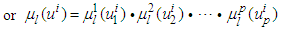
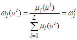
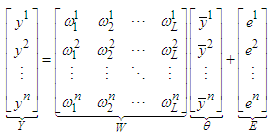
- Generally, fuzzy inference systems (FIS) can be systematically constructed from “pure” input–output data. All methods are based on the optimization of a cost function to minimize the “distance” between the predictions of the FIS and the output data. The main differences among the methods are the initialization and the adjusted parameters.The basic FRBL scheme was original proposed by Wang [37]. In this paper, some simple modifications are proposed and these modifications are related to the consequence calculations. In the proposed modifications: the position, the shape and the distribution of the membership functions are choices for the designer rather than being fixed. Further, the rule-based logic is initialized through clustering based on experimentally acquired data and the proposed method finds only the consequences of the rules.Supposed that a sequence of input–output
 for
for  data is collected, the inputs
  and the output
  . The subset
  is a portion of the space
  and is defined as
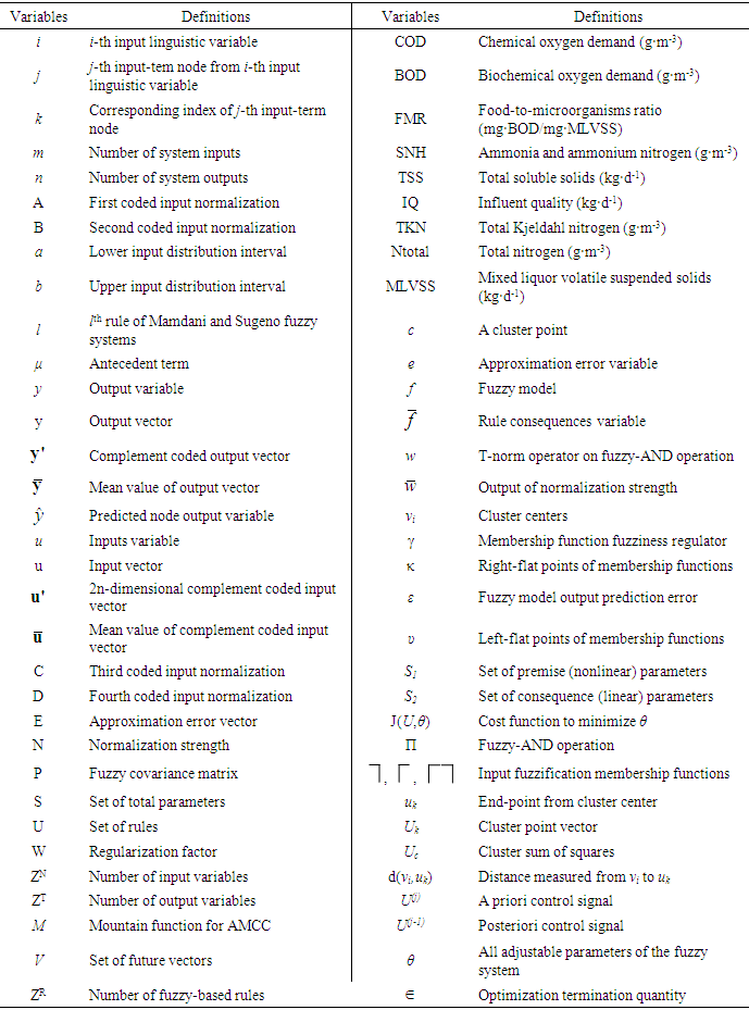
 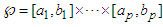 . The procedure to construct the model is laid out in the following [12,13,16–21]:1). For each of the p inputs of the system distribute over the interval
  and ni membership functions. The shape, position and distribution can be arbitrarily specified. The only condition is that the full interval must be covered and at least two membership functions should be placed on each point of the input domain. However, note that the shape and the distribution affects the smoothness and the accuracy of the approximation.2). Generate the rules using all possible combinations among the antecedents and the AND-operator (choosing in advance “min” or “product” operator).(i). The rule l of the rules for Mamdani fuzzy systems is IF
  is
is  AND … AND
  is
is  THEN
THEN  is
is  (ii). The rule l of the rules for Takagi–Sugeno fuzzy systems is IF
  is
is  AND … AND
  is
is  THEN
THEN 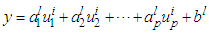 3). Calculate the inference of each rule. For rule l of the form
 | (1) |
 | (2) |
 | (3) |
 | (4) |
 for
for  such that
  . Observe that (3) can be written as
 | (5) |
 | (6) |
 | (7) |
 and
and  for
for  such that
  . Using the reasoning applied for the Mamdani fuzzy models, Equation (4) can be written as:
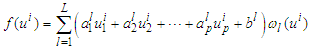 | (8) |
 has the same form shown in Equation (6). Again, the n output values can be represented as the vector Y in terms of the inference process as
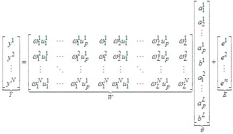 | (9) |
 | (10) |
 | (11) |
2.2. The HANFA–ART with ACA Network Architecture
- The proposed HANFA-ART with ACA network consists of six layers as shown in Figure 1. The proposed network architecture employs two major algorithms for parameters adjustment and learning (i.e. the ARLS and MLMA) and one algorithm for automatic structure learning (i.e. the fuzzy-ART). In the following, we briefly describe the operation of each layer. A descriptive representation of a m-inputs and n-outputs HANFA-ART with ACA network architecture with 4-fuzzy rules is shown in Figure 1. The code segment that executes the Fuzzy-ART algorithm is adopted (with the necessary modifications) from the well-structured, reliable and tractable Fuzzy-ART [13].Unlike the common and most widely used ANFIS architectures including the one implemented in MATLAB / Simulink® [25], the version adopted in this work was first proposed in Lin and Lin [12] and later modified by Garrrett [13]. It is called the adaptive neuro-fuzzy inference system (ANFIS) based on adaptive resonant theory (ART). Instead of the conventional five layers, the proposed HANFA-ART with ACA has six layers as shown in Figure 1. For completeness, consistency and simplicity, each of these six layers is described below with their accompanying mathematical descriptions.
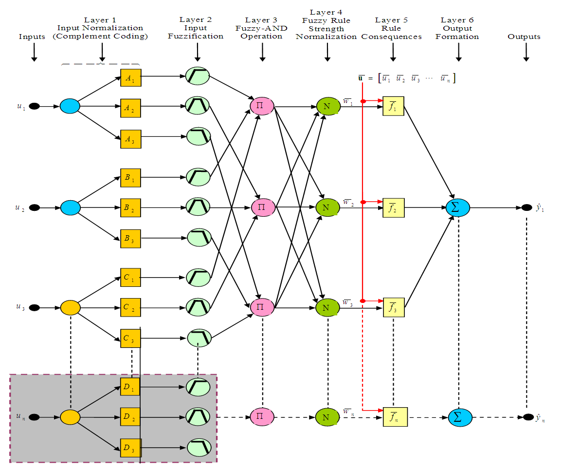 | Figure 1. The HANFA-ART with ACA network architecture |
 with its 2n-dimensional complement coded form u' such that:
 | (12) |
 . Complement coding helps avoiding the problem of category proliferation when using fuzzy-ART for data clustering. Having this in mind, we can write the I/O function of the first layer as follows:
 | (13) |
 | (14) |
 and
and  are respectively the left-flat and right-flat points of the trapezoidal membership function of the j-th input-term node of the i-th input linguistic variable.
  is the input to the j-th input-term node from the i-th input linguistic variable (i.e.
  ). Also, the function
  is defined as:
 | (15) |
 | (16) |
 | (17) |
 and implements the linear function:
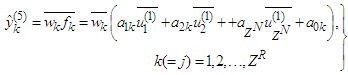 | (18) |
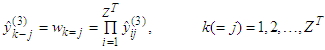
 is the normalized activation value of the k-th rule calculated with the aid of Equation (18). Those parameters are called the consequent parameters or linear parameters of the HANFA-ART system and are regulated by the proposed ARLS algorithm [31–33].Layer No.6 - Output LayerFor the proposed HANFA-ART system, this layer consists of one and only node that creates the network’s output as the algebraic sum of the node’s inputs:
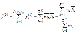 | (19) |
2.3. The Adaptive Clustering Algorithms (ACA)
- Until now, the fuzzy sets of the input domains have been placed on their initial positions which is usually equally distributed from the experimental data. Two choices are available for re-positioning these input domains, namely: 1) the number of membership functions and 2) their initial distribution. However, the methods based on clustering aim to obtain both parameters at the same time, the number of fuzzy sets needed to make the function approximation and their distribution along the input domains.Clustering methods are a set of techniques to reduce groups of information U represented as p-dimensional vectors into characteristic sets
 characterized by feature vectors
  and membership functions
  .The methods based on clustering are considered as data-driven methods [14,16–21]. The main idea of these methods is to find structures (clusters) among the data according to their distribution in the space of the function and assimilate each cluster as a multidimensional fuzzy set representing a rule. The cluster prototypes can be either a point (to construct Mamdani models) or a hyperplane (to construct Takagi–Sugeno models) [16–21].The fuzzy inference system is constructed by means of projecting the clusters into the input space and approximating the projected cluster with a one-dimensional fuzzy set. The advantage of these methods is that the membership functions can be automatically generated such that only the parameters of the clustering algorithms (number of clusters and distance function) can be arbitrarily chosen. According to the type of model to be constructed, the clustering method can be slightly different. In the next few sub-sections, the clustering algorithms as applied to the Mamdani and the Takagi–Sugeno fuzzy models are presented.
2.3.1. The K-Means Clustering Algorithms
- The hard-partitioning methods are simple and popular, though its results are not always reliable and these algorithms have numerical problems as well [14,25]. From an
 dimensional data set, K-means and K-medoid algorithms allocates each data point to one of c clusters to minimize the within-cluster sum of squares [14]:
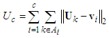 | (20) |
 | (21) |
 . The K-means clustering algorithm is used to initialize the data clustering process. This initial clustering by the K-means algorithm sets the initial partitioning of the given data set from the initial distribution.
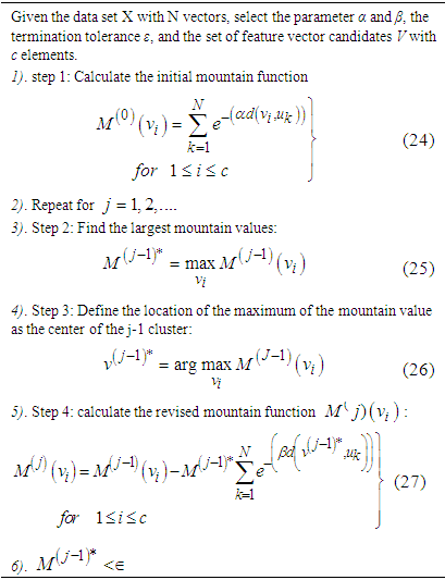
2.3.2. Adaptive Mountain Climbing Clustering (AMCC) Algorithm
- In the AMCC algorithm, a super set of the feature vectors V is proposed in advance, then some vectors are selected according to the value of the mountain function calculated for the given vector
 . The mountain function is defined as [17,18]:
 | (22) |
 is a positive constant and
  is a distance measure from
  to
to  and it is typically but not necessarily:
 | (23) |
|
 . This has also been shown not to be very efficient for large data sets [1–3,12–21]; and2). Take a grid (arbitrary) defined in the interval where the points of u are defined. This has also been shown not to be very efficient for vectors defined on a large-dimensional space [1–3,12–21].Compared with other clustering methods [14–16], the mountain clustering method has as its main advantage the fact that the number of clusters does not need to be defined in advance. The implementation of the adaptive mountain clustering algorithm is summarized in Table 2.
2.3.3. Adaptive Gustafson and Kessel Clustering (AG-KC) Algorithm
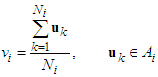
- The adaptive Gustafson and Kessel clustering algorithm is based on the minimization of the cost function [18]:
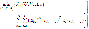 | (28) |
 with the information,
  is the set of feature vectors,
  is a set of c norm-inducing matrices and
  is the fuzzy partition matrix, defined as an element of the set:
 | (29) |
 row of the fuzzy partition matrix contains the membership values of the vectors u to the
  fuzzy set. Observe that the cost function can be arbitrarily small by reducing the norm of each
  . For this reason a constraint is introduced to preserve the norm of
 Applying the Lagrange multipliers to the above optimization problem of Equation (29) generates the following expression for
  :
: | (30) |
 is the fuzzy covariance matrix:
 | (31) |
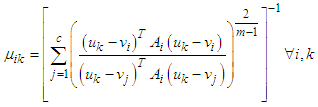 | (32) |
 are calculated as
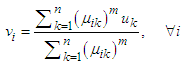 | (33) |
|
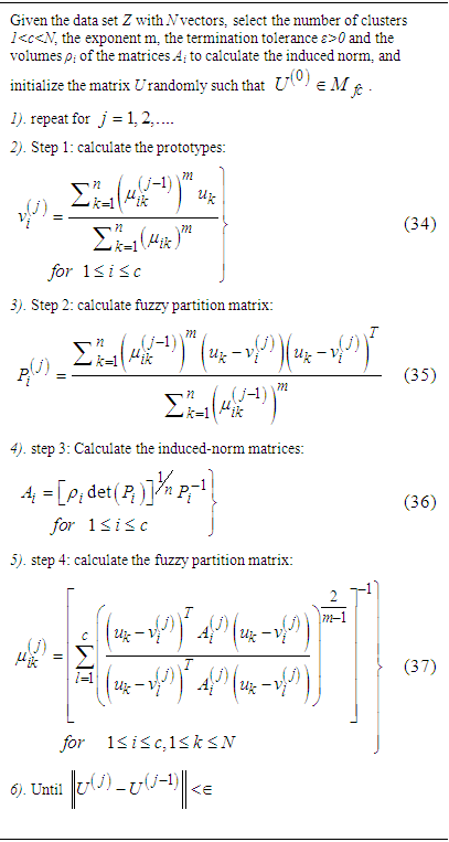
 is equal to one of the prototypes
  the Equation (37) becomes singular. For this case the membership value
  for this vector is equal to one and zero for all the other entries in the
  row of U. The parameter m is a very important parameter. As
  , the means of the clusters tend to the mean of the set U.
2.4. The Adjustable Parameters of the HANFA-ART with FRBL System
- This method requires the definition of the number of membership functions and their shape. Normally the AND function is fixed to be the “product” because an analytical expression for the gradient of the cost function is needed. The initial position of the membership functions is another element that must be chosen. The method proceeds as follows:1). For each of the p inputs of the system, distribute over the interval [ai, bi] and Ni membership functions; the shape, the initial positions and the distribution can be chosen arbitrarily as just discussed in Section 2.3. The membership functions must cover the input interval, and at least two membership functions should be placed on each input domain.2). Generate the rule base using all possible combinations among the antecedents and the AND operator using “product”.3). Initialize the value of the consequences using prior knowledge, least squares or recursive least squares.4). Optimize the value of the consequences
 and the parameters of the membership functions. The criteria will be to minimize the cost function described in the previous section, but now the optimization will also adjust the membership functions of the antecedents. The cost function can be described as
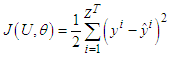 | (38) |
 and θ is a vector representing all the “adjustable” parameters (consequences, parameters of the membership functions) of the fuzzy system
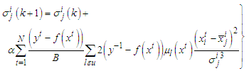
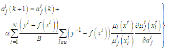
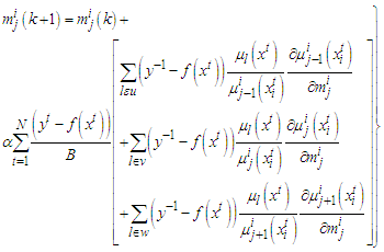
  . The problem will be the minimization of the cost function J. This minimization is a nonlinear and non-convex optimization problem. The objective is to obtain an “acceptable” solution and not necessarily “the global minima” of this cost function of Equation (38).Different schemes for optimization can be applied to find this solution but the probably simplest method is the gradient descent method [31–33,38–40]. This method consists of an iterative calculation of the parameters oriented to the negative direction of the gradient [38–40]. The explanation behind this method is that by taking the negative direction of the gradient, the steepest route toward the minimum will be taken. This descent direction does not guarantee convergence of the scheme and it is for this reason that the parameter α is introduced which can be modified to improve the convergence rate and properties [31–33,38–40]. Some choices of α are given by Newton and quasi-Newton methods [9,38–40].In this paper, two algorithms have been adopted and adapted for estimating and updating the adjustable parameters (i.e. the consequences parameters and the parameters of the membership functions) of the proposed HANFA-ART with ACA system [31–33]. These two algorithms are: 1). an efficient recursive least squares algorithm called the adaptive recursive least squares (ARLS) algorithm, and 2). an efficient gradient descent algorithm called the modified Levenberg-Marquardt algorithm (MLMA) [31,32].
2.5. Training of the Proposed HANFA-ART with ACA
- Next, how the HANFA-ART with ACA is trained to learn the premise and consequent parameters for the membership functions with the associated rules is considered. There are numbers of possible approaches but the learning algorithm proposed by Jang and co-workers which uses a combination of steepest descent and least squares estimation (LSE) has been widely used with several challenges [38–40]. However, these challenges have been shown to be very complicated but a systematic implementation to overcome these challenges is presented in the remaining of this paper for the proposed HANFA-ART with ACA.It can be shown that for the network illustrated in Figure 1, if the premise parameters are fixed, the output is linear in the consequent parameters. Then, the total parameters set can be split into three sets: S = set of total parameters, S1 = set of premise (nonlinear) parameters, and S2 = set of consequent (linear) parameters. Thus, the HANFA-ART with ACA uses a two-pass learning algorithms:1). Forward Pass: Here S1 is unmodified and S2 is computed using an adaptive recursive least square (ARLS) algorithm described in [31–33]; and2). Backward Pass: Here S2 is unmodified and S1 is computed using a special gradient descent algorithm called the MLMA algorithm described in [31,32].So, the proposed hybrid learning algorithm uses a combination of steepest descent algorithm (i.e. the proposed MLMA) and a recursive least squares algorithm (i.e. the proposed ARLS) to adapt the parameters in the adaptive network. The summary of the learning process is given below:(1). The Forward Pass: This propagates the input vector through the network layer by layer as followsi). Present the input vector;ii). Calculate the node outputs layer by layer;iii). Repeat for all data à A and y formed;iv). Identify parameters in S2 using the ARLS algorithm; andv). Compute the error measure for each training pair.(2). Backward Pass: In this case, the error is sent back through the network in a manner similar to the back-propagation but it is implemented here by the MLMA algorithmi). Use the MLMA algorithm to update parameters in S1; andii). For given fixed values of S1, the parameters in S2 found by this approach are guaranteed to be the global optimum [31–33].
2.6. Summary of Algorithms for Mamdani and Takagi–Sugeno Fuzzy Models
- The summary of the clustering algorithms incorporating the ARLS and the MLMA algorithms for calculating the consequences parameters that are not covered by the cluster using ARLS and then applying the MLMA to adjust the antecedents parameters appropriately as given in the following sub-sections.
2.6.1. Algorithm for Mamdani Fuzzy Models
- Step 1: Collect the data and construct a set of vectors
 where u and y are the inputs and the output of the function respectively. Observe that it is assumed here that
  and
and  ;Step 2: Search for clusters using the combination of the K-means and the AMCC algorithms for problems where the dimension of the input space is small;Step 3: Project the membership functions from the partition matrix U into the input space;Step 4: Approximate the appropriate projected membership function using convex membership functions such as triangular, Gaussian, polynomial, trapezoidal, etc. as described in Appendix A, B and C [18];Step 5: Construct the rules with the appropriate projected membership functions;Step 6: Calculate the consequences using recursive least squares using the ARLS algorithm; andStep 7: Adjust the parameters of the antecedents using gradient descent-based MLMA.
2.6.2. Algorithm for Takagi–Sugeno Models
- Step 1: Collect the data and construct a set of vectors
 where u and y are the inputs and the output of the function respectively. Observe that it is assumed here that
  and
and  ;Step 2: Search for clusters using the combination of the K-means and the AG-KC algorithms;Step 3: Check for similarities among the clusters. Do two clusters describe a similar hyperplane?;Step 4: Project the membership functions from the partition matrix U into the input space;Step 5: Approximate the appropriate projected membership function using convex membership functions such as triangular, Gaussian, polynomial, trapezoidal, etc. as described in Appendix A, B and C [18];Step 6: Construct the rules with the projected membership functions;Step 7: Generate the consequences using the covariance matrices of each cluster;Step 8: Calculate the consequences that are not covered by the clusters using recursive least squares using the ARLS algorithm; andStep 9: Adjust the parameters of the antecedents (if needed) using gradient descent-based MLMA.
3. Applications of HANFA-ART with ACA for Classification, Prediction and Control
3.1. Classification of Meningitis Using HANFA-ART with ACA Algorithm with Mamdani Fuzzy-Type Model
3.1.1. Problem Description
- Meningitis is an acute inflammation of the protective membranes covering the brain and spinal cords, known collectively as meninges [41]. The inflammation may be caused by infection with bacterial, viral, fungal, parasitic, amebic, tuberculosis, non-infectious and other microorganisms (such as fungi, protozoa, etc) and less commonly by drugs [42]. The most common symptoms of meningitis are headache and neck stiffness associated with fever, confusion or altered consciousness, vomiting and inability to tolerate light (photphobia) or loudness (photophobia). Children usually show non-specific symptoms such as drowsiness and irritability [43]. Meningitis is a form of meningococcal disease which is very serious [41,42]. About 10 to 15% of people with meningococcal disease die even with appropriate antibiotic treatment. Of course those who recover have problems with their nervous system; up to 20% suffer from some serious after-effects, such as permanent hearing loss, limb loss, brain damage or suffer seizure or strokes [41–43].Meningitis can be life threatening because of the inflammation proximity to the brain and spinal cord; therefore, the condition is classified as medical emergency [41–43]. This leads to the requirement of developing a new technique which can detect and classify the occurrence of meningitis giving some symptoms. This will help in better diagnosis in order to reduce the number of meningitis patients.
3.1.2. Formulation of the Meningitis Classification Problem
- The proposed HANFA-ART with ACA algorithms is implemented here for the classification of the 18 attributes that could cause meningitis classified into six (6) classes namely: abscess which corresponds to “Class 1”, bacteria which corresponds to “Class 2”, bacteria E which corresponds to “Class 3”, virus which corresponds to “Class 4”, virus E which corresponds to “Class 5” and tuberculosis which corresponds to “Class 6”. The 18 attributes include: 1) cold, 2) headache, 3) fever, 4) nausea, 5) loc, 6) seizure, 7) BT, 8) stiff, 9) GCS, 10) WBC, 11) CRP, 12) ESR, 13) CSF cell, 14) cell poly, 15) cell mono, 16) CSF pro, 17) CSF pro, and 18) age. A total of 140 data were collected for the 18 attributes just mentioned and their respective plots are shown in Figure 2 (a) – (f); while their six respective classes for the 18 attributes over the 140 experimental data set is shown in Figure 3. The two algorithms are: 1) adaptive neuro-fuzzy inference system trained with back-propagation (ANFIS with BPM) and 2) the proposed HANFA-ART with ACA.
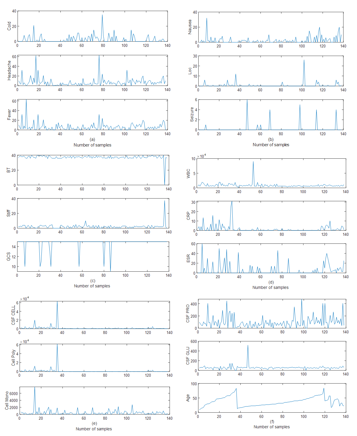 | Figure 2. The 18 attributes: (a) cold, headache and fever, (b) nausea, loc and seizure, (c) BT, stiff and GCS, (d) WBC, CRP and ESR, (e) CSF cell, cell poly and cell mono, and (f) CSF pro, CSF pro, and age |
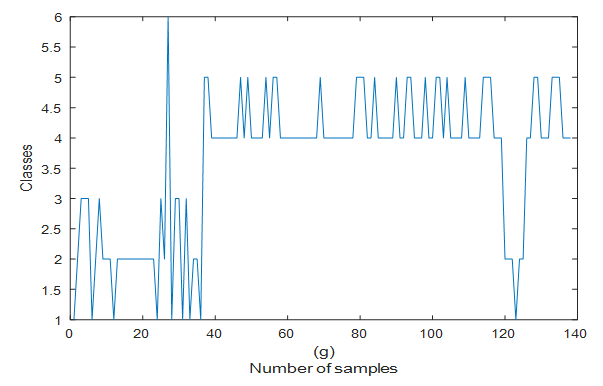 | Figure 3. The six respective classes for the 18 attributes over the 140 experimental data set |
3.1.3. Implementation of the Meningitis Classification Problem
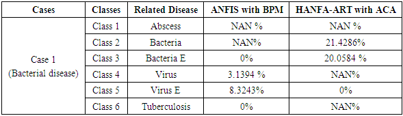
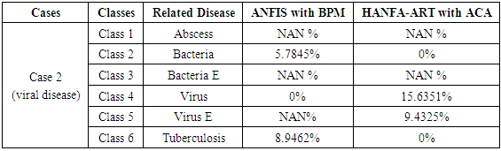
- Case 1: Bacterial Related Disease for the Cause of MeningitisThe implementation of these two algorithms (ANFIS with BPM and HANFA-ART with ACA) presented in this paper for a known cause of illness is carried out. The input data set is characterized by bacteria and the objective here is to evaluate the ability of the algorithms to classify the data set into this category and compared the obtained classification with a standard adaptive neuro-fuzzy inference system (ANFIS) trained with backpropagation with momentum (BPM) algorithm which is collectively called here as ANFIS with BPM [2,20,44].Upon the implementation of the two algorithms, the result of Table 4 and the comments of Figure 4 (a) and (b) were obtained. The results of Figure 4 show the classification of a bacterial disease based on (a) ANFIS with BPM and (b) HANFA-ART with ACA. As it can be seen from Table 4 based on the results obtained using HANFA-ART with ACA, the major symptom is a bacterial related disease (Class 2) with 21.4286% followed by 20.0584% of a bacteria E related disease (Class 3) and a NAN% of virus related disease. Note although the 0% for virus may mean nothing but it is a value which indicate the absence of virus which when compared to NAN (Not A Number) which is assumed to have no effect nor contribute to the individual’s illness.
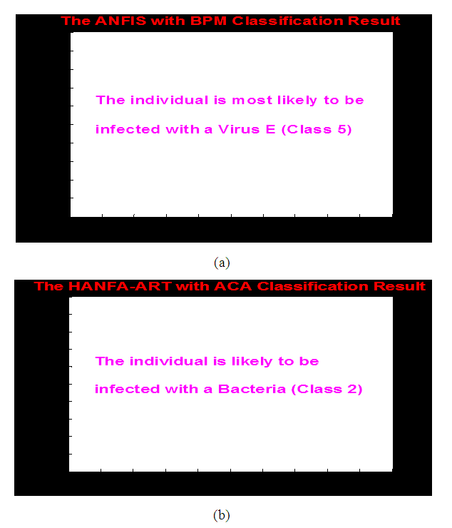 | Figure 4. Results for the classification of a bacterial disease based on (a) ANFIS with BPM and (b) HANFA-ART with ACA |
|
|
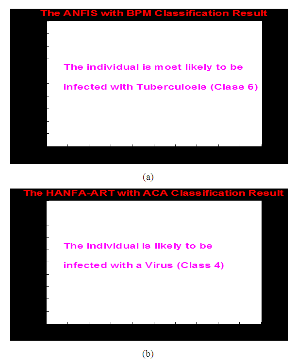 | Figure 5. Results for the classification of a viral disease based on (a) ANFIS with BPM and (b) HANFA-ART with ACA |
|

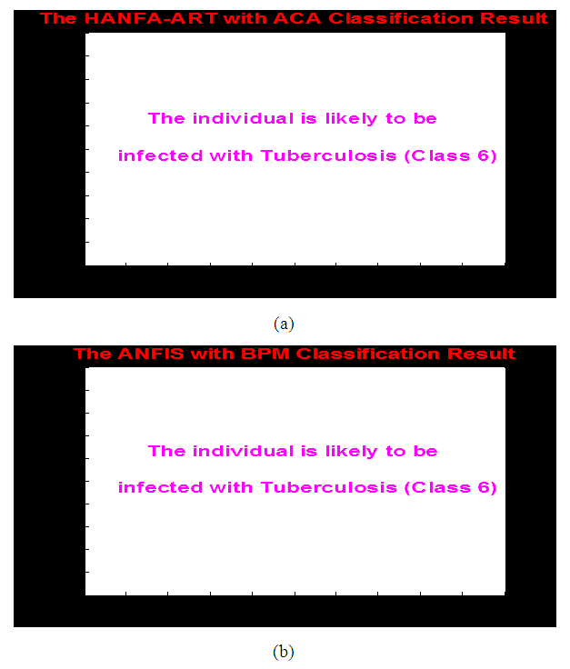 | Figure 6. Results for the classification of a tuberculosis related disease based on (a) ANFIS with BPM and (b) HANFA-ART with ACA |
3.1.4. Summary of the Results for the Meningitis Classification Problem
- The main task of this sub-section has been on how to correctly classify a disease (infection) or diseases (infections) in terms of 18 different attributes (symptoms) which could lead to meningitis. The 18 different attributes were classified into six (6) different classes of diseases (infections). The total data representing the 18 attributes is 2,520 (i.e. 140 x 18) which in addition to the 140 classes (i.e. 140 x 1) gives a grand total of 2660 data used in this study.To this end, an HANFA-ART with ACA algorithm has been proposed in this paper. In order to evaluate the performance of the proposed algorithm, a second algorithm called ANFIS with BPM algorithm has also been presented. The performance of the proposed algorithm for a classification problem have shown acceptable results and are in agreement with the expected results except for the ANFIS with BPM which seldom gives good result. This is not surprising since networks trained with back-propagation related algorithm usually give poor performance since back-propagation algorithm on its own has several problems such as poor robustness, poor convergence property, long training cycles, large network parameters, etc.The classification performance results obtained by the HANFA-ART with ACA demonstrate the classification efficiency and capability of the proposed algorithms. In order to place a benchmark, 500 iterations (epochs) was used throughout all the simulations and the number of input-to-hidden neurons were limited to 15 neurons. The simulation results show high prediction and classification accuracies when compared to the characteristics of the input data. The two algorithms proposed, implemented and demonstrated in this work can be adapted in hospitals and medical centers for immediate diagnosis based on the reports from patients.
3.2. Setpoint Determination for AS-WWTP Influent Pump Control Using a Takagi-Sugeno Fuzzy-Type Model
3.2.1. Description of the AS-WWTP System
- The activated sludge model is a generic name for a group of mathematical methods to model activated sludge waste water treatment plant (AS-WWTP). The research in this area is coordinated by a task group of the International Water Association (IWA) [31,45]. The Activated sludge models are used in scientific research to study biological processes in hypothetical systems. They can also be applied on full scale wastewater treatment plants for optimization, when carefully calibrated with reference data for sludge production and nutrients in the effluent [31,45–48]. Modelling the activated sludge process has an important role in implementing efficient control actions for better process performance. However, the reliability of the proposed models depends on an increasing number of kinetic and stoichiometric parameters, which to a large extent depend on the characteristics of the actual wastewater and must therefore be experimentally determined.There is little doubt that control strategies can be evaluated by model simulation. However, the protocol used in the evaluation is critical. To make unbiased comparisons, the influent pump control strategy must be evaluated under the simulation benchmark condition. Also, the effect of the control strategy must be compared to a fully defined and suitable reference output. The ‘simulation benchmark’ defines such a protocol and provides a suitable reference outputs for operational performance assessment [31,45–48].The simulation benchmark plant design comprises five reactors in series with a 10-layer secondary clarifier or settler as shown in the schematic representation of the layout of Figure 7 while the Simulink implementation of the benchmark model for experimental data generation with constant influent is shown in Figure 8. The detailed description and explanation of the AS-WWTP simulation benchmark and the Simulink model can be found in [31,45–48].
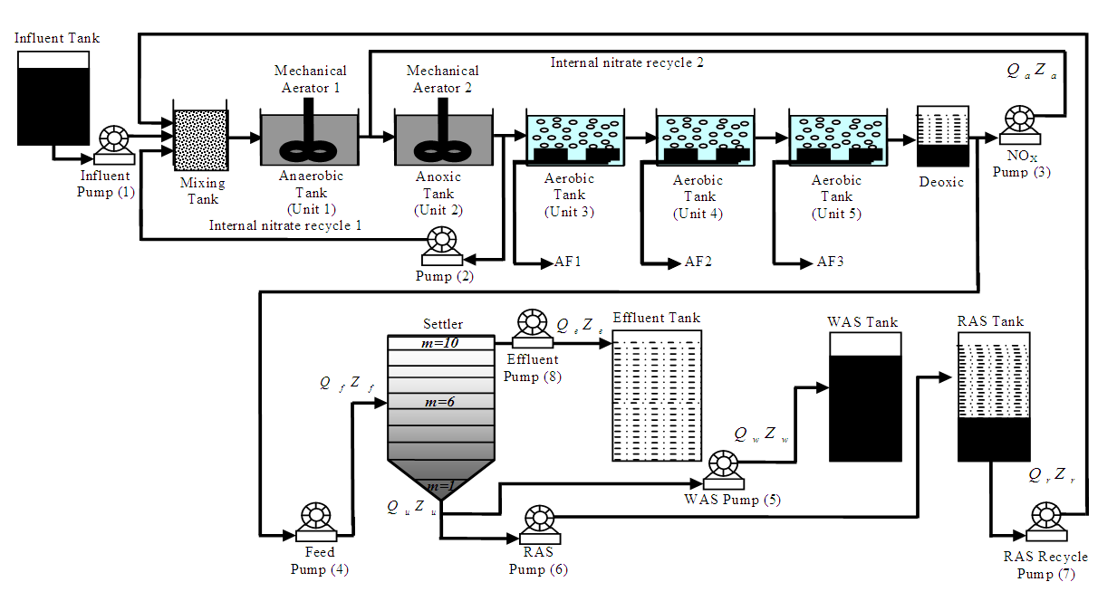 | Figure 7. The schematic of the AS-WWTP process [31,46–48] |
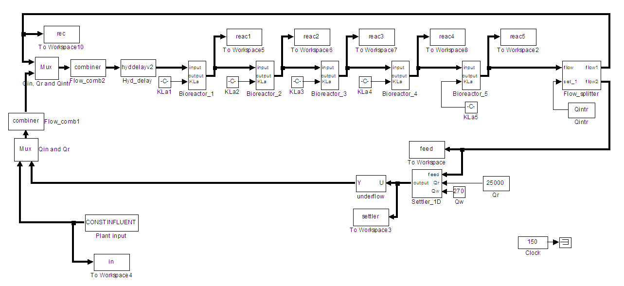 | Figure 8. Open-loop steady-state benchmark simulation model for the AS-WWTP with constant influent [31,46–48] |
3.2.2. Formulation of the AS-WWTP Influent Pump Control Problem
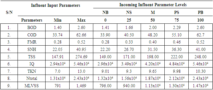
- Here an attempt is made to use the HANFA-ART with ACA for the prediction and adaptive control of the influent pump (pump 1) of an AS-WWTP based on the setpoint generated by the HANFA-ART with ACA based the rules shown in Table 7. The constraints for the influent pump operation is between 0 and 1.20 x 10⁵ revolution per day (rev/day) while the influent flow into the first biological reactor at a typical rate of 2.0 x 10⁴ mg·l-1. [31,45–48] The various units for the eight parameters in Table 7 are given in Table 1. The minimum and maximum values are split into five levels Negative Big (NB), Negative Small (NB), Medium (M), Positive Small (PS), and Positive Big (NB) which indicates the appropriate setpoint for the influent pump control. Note that each of the 8 input parameters has 5 levels which give 8 x 5 x 5 = 200 possibilities of fuzzy rules that are used to manipulate the influent pump at each sampling time. A brief manipulation of the influent pump based on these parameters is highlighted in the following:1). When all the values are met, then pump one is widely open i.e. Positive Big (PB);2). When all other conditions are met but one of the parameter has a lesser value than the required value given by COST 624, then pump1 is open wide i.e. PB provided that FMR is exact;3). When at most three of the parameters has a lesser value while others meet the demand of the COST 624 for pump1, pump1 is partially open, i.e. Positive Small (PS) provided that FMR is exact. Another condition is that when all conditions are met but any one of the parameters having value above the demand, the pump is again allowed to be partially opened i.e. Positive Small (PS) provided that FMR, TSS and MLVSS are exact;4). When more than three of the parameters do not meet the COST 624 demand, pump1 is partially closed i.e. Negative Small (NS); and5). When more than one of any of the parameters have values higher than necessary as given by the COST 624, pump1 should be almost closed i.e. Negative Big (NB).
|
3.2.3. Implementation of the HANFA-ART with ACA for Setpoint Determination for AS-WWTP Influent Pump Control
- The Simulink implementation of the HANFA-ART with ACA for the setpoint determination for the prediction and adaptive control of AS-WWTP influent pump is shown in Figure 9. As can be seen in Figure 9, the AS-WWTP constant influent state parameters are fed through a summer with the predicted AS-WWTP influent parameters in a negative feedback mode at the first sampling instant. The influent parameters from the summer forms the inputs to the HANFA-ART with ACA Takagi-Sugeno type fuzzy model which employs the rules defined by Table 7 to determine the appropriate setpoint for the influent pump output prediction, tracking and control against a desired reference influent pump output as shown in Figure 9.
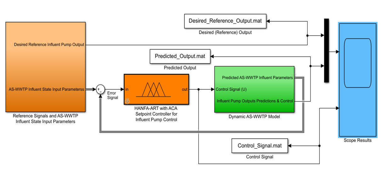 | Figure 9. The Simulink implementation of the HANFA-ART with ACA for setpoint determination for the control of AS-WWTP influent pump |
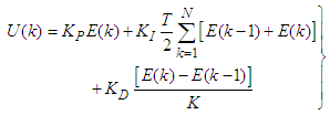 | (39) |
 is the error between the desired reference
  and predicted output
  , and N is the number of samples. The minimum and maximum constraints imposed on the PID controller to penalize changes on the AS-WWTP pump control inputs
  and outputs
  are given as:
 | (40) |
3.2.4. Simulation and Discussion of Results Setpoint Determination for the AS-WWTP Influent Tank Control Problem
- The simulation results of the output predictions, tracking and adaptive control of the AS-WWTP influent pump based on accurate setpoint determination is shown in Figure 10 where (a) shows the comparison of the HANFA-ART with ACA and the PID controller for output predictions, tracking and adaptive control of the influent pump against the desired reference output of the influent pump while Figure 10(b) shows the output prediction errors between the predicted output by the PID controller and the HANFA-ART with ACA against the desired reference outputs; and Figure 10(c) compares the control signal generated by the PID controller and HANFA-ART with ACA for the adaptive control of the influent pump in order to tack the desired output. The control signal is the energy required to manipulate the influent pump to achieve excellent performance to tack with the desired reference output based on the setpoint.It is evident in the simulation results of Figure 10(a)-(c) that the HANFA-ART with ACA algorithm exhibit excellent setpoint determination which enhances the good output prediction, tracking and adaptive control of the influent point when compared the results obtained by the PID controller. The superior performance of the HANFA-ART with ACA over the PID controller is further justified by the maximum output prediction errors of 123.51 rev/day when compared to the maximum output prediction errors of 419.92 obtained by the PID controller. The minimum and maximum control effort by HANFA-ART with ACA varies between 36.36 and 1.64 x 10³ rev/day respectively compared to the excessive minimum and maximum control effort of between 151.85 and 2.33 x 10³ rev/day respectively control energy required by the PID controller.
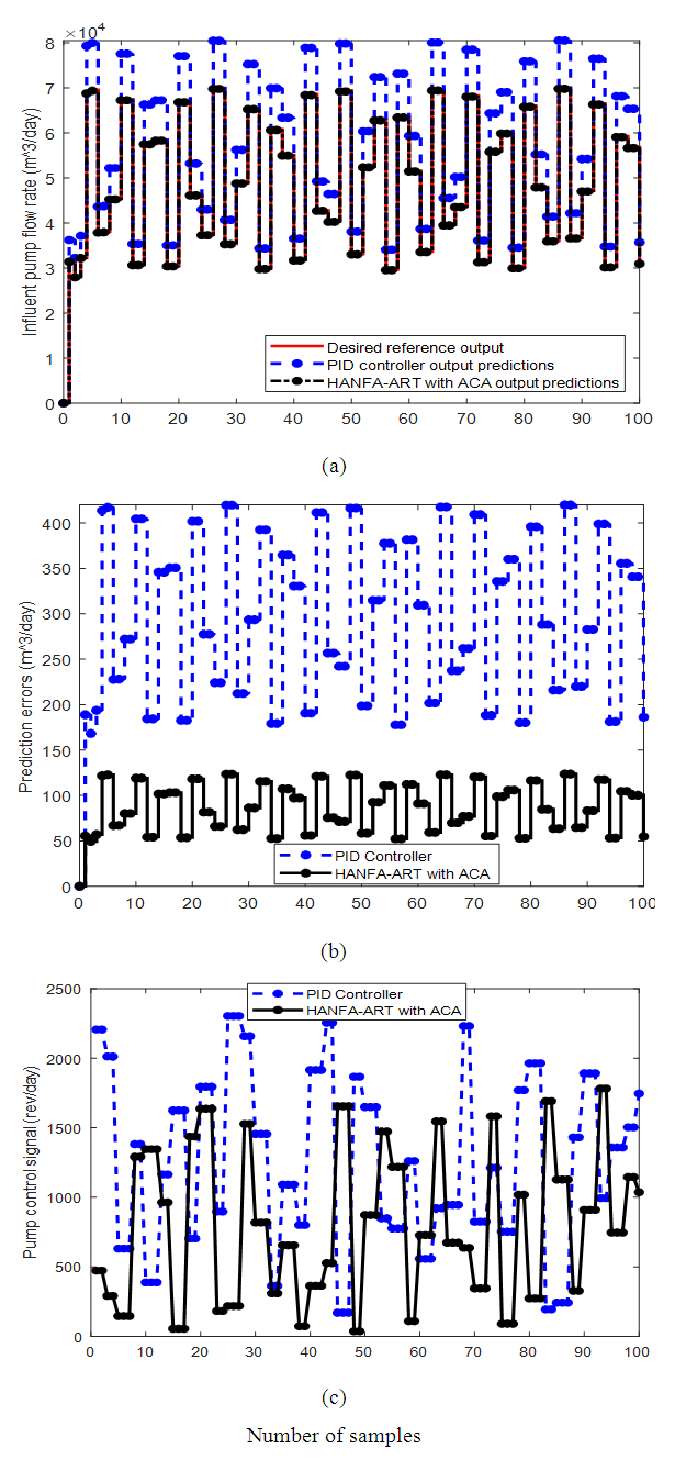 | Figure 10. Output predictions, tracking and adaptive control of the AS-WWTP influent pump based on accurate setpoint determination: (a) comparison of the adaptive control and tracking of the desired reference output by the PID controller and HANFA-ART with ACA, (b) PID controller and the HANFA with ACA output prediction errors, and (c) control signal generated by PID controller and the HANFA-ART with ACA for the adaptive control of the influent pump |
4. Conclusions
- The architecture and learning procedures for the HANFA-ART with ACA presented above is an adaptive fuzzy inference system implemented in the framework of adaptive neural networks and adaptive resonant theory as well as adaptive clustering algorithm. By using the proposed hybrid learning procedures, the proposed HANFA-ART with ACA has been able to construct an input-output mapping based on both human knowledge (in the form of fuzzy if-then rules) and adaptive input-output models.The efficiency of the proposed HANFA-ART with ACA has been validated with two problems, namely: (i) classification of meningitis related diseases using HANFA-ART with ACA algorithm using the Mamdani-type fuzzy-type model, and (ii) setpoint determination for the output prediction, tracking and adaptive control of an AS-WWTP influent pump using Takagi-Sugeno fuzzy-type model.The HANFA-ART with ACA algorithm clearly outperforms the standard ANFIS with BPM for the meningitis problem based on the excellent and accurate classification of the related disease that could be responsible for the meningitis.Unlike conventional model reference adaptive control (MRAC) where plant parameters are adjusted to obtain the plant model for the controller design amid tight constraints or in model predictive control (MPC) where an explicit model of the plant is required for the controller design amid tight constraints [9,51]. However, the technique proposed and implemented in this work using the HANFA-ART with ACA is completely different. The idea here is to represent the plant behaviour as in Table 7 and the HANFA-ART with ACA is combined with the Takagi-Sugeno fuzzy-type in closed-loop for excellent output predictions, tracking of desired reference trajectory and adaptive control performance of the AS-WWTP influent pump as can be seen evidently in Figure 10(a)-(c) justified with small output prediction errors and minimum control effort when compared the well-celebrated PID controller.It is worthwhile to note that clustering of numerical data forms the basis of many system modeling and identification, prediction and classification algorithm. The purpose of clustering such as the subtractive clustering used in this work is to identify natural groupings of data set to produce a concise representation of system’s behaviour or trend within the data set.Thus data clustering presents computationally intensive task. It is recommended that parallel computing be used for the implementation of the algorithms proposed in this work for real-time applications.The optimization algorithms used in this work are all classical optimization algorithms which are gradient descent algorithms. The implication is that they are based on sequential gradient-based searching technique and a global optimum may not be easily obtained together with huge computational overhead for large multivariable data set or systems. Hence, the use of evolutionary optimization techniques such as any variation of genetic algorithms could alleviate this problem.Other broad areas of applications of the proposed classification, prediction, tracking and adaptive control algorithms presented in this work are inexhaustible and should be investigated.
Appendix A: Gradient Updates for Membership Functions
- A.1. Gradient Update for Gaussian Membership FunctionsThe parameterization of the membership functions is given by
 | (A-1) |
 will be given by
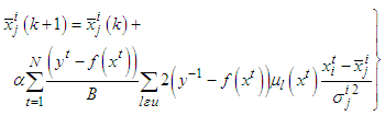 | (A-2) |
 | (A-3) |
 .A.2. Gradient update for Trapezoidal Membership FunctionsAssuming the parameterization given in the expression
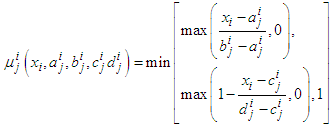 | (A-4) |
 | (A-5) |
 | (A-6) |
 | (A-7) |
 | (A-8) |
 is the set of rules that includes the function
  in the antecedents and
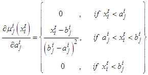 | (A-9) |
 | (A-10) |
 | (A-11) |
 | (A-12) |
 . This adaptation rule can be applied to triangular membership functions by just making
  .
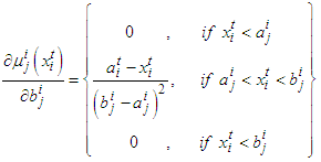
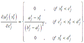
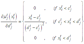
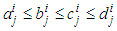
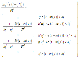
.Appendix B: Gradient Update for Triangular Membership Functions with 0.5 Overlap
- The membership functions are parameterized by using only their modal values. This parameterization not only preserves the overlap but also reduces the number of parameters to be turned. Triangular membership functions are parameterized by the position of their three vertices; but the condition of overlap 0.5 makes the lower right vertex of one membership functions to be at the same position as the modal value of the next membership function. So, instead of turning three parameters (the vertices), only one parameter is turned for each membership function.The parameterization for a triangular membership function using the modal values as parameters is
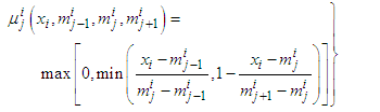 | (B-1) |
 | (B-2) |
 and
and  , respectively, and with
 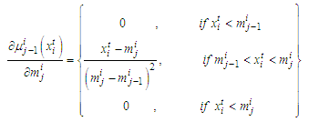 | (B-3) |
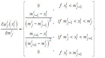 | (B-4) |
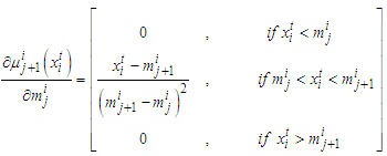 | (B-5) |
 is preserved.
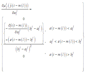
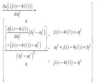
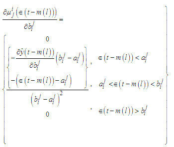
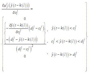
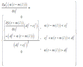
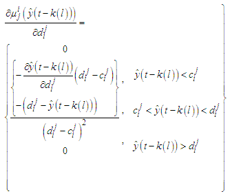
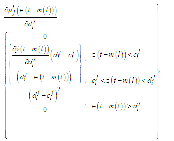
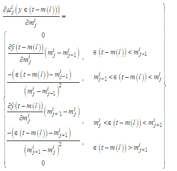
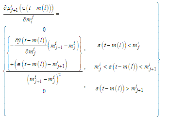
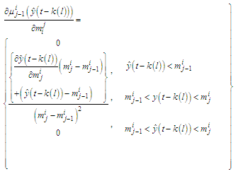
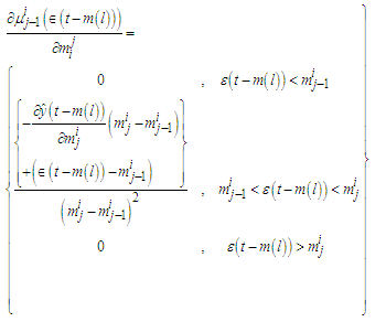
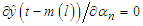
Appendix C: Gradient Expressions for Identification of Fuzzy Models with Membership Functions
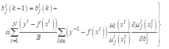
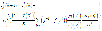
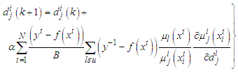
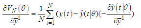
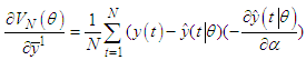
- C.1. Gradient Expressions for Identification of Fuzzy ModelsThe gradients derived in this appendix are useful in the optimization of dynamic models. The cost function to be minimized is the quadratic cost function, which is defined as
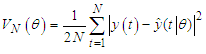 | (C-1) |
 is the output of the “real” system at time t,
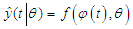 | (C-2) |
 is the output of the constructed model parameterized by the vector
  . The vector
  describes the membership functions and the position of the singletons in the consequences and
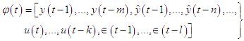 | (C-3) |
 | (C-4) |
 | (C-5) |
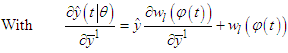
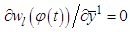 and the expression for the gradient will be the same used for static function approximation. The term
 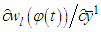 is dependent from previous gradient values and must be generated dynamically.
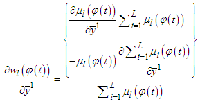 | (C-6) |
 | (C-7) |
 with delay
  and
and  represents the set of inputs related with the regressors
  with delay
  , and
, and 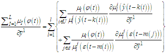 | (C-8) |
 and
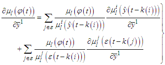
and 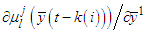 will have the following expressions:C.2.1. Gradient for the Singleton Consequences with Gaussian Membership Functions For Gaussian membership functions using the parameterization presented in (A-1):
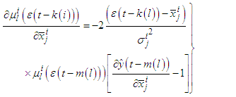
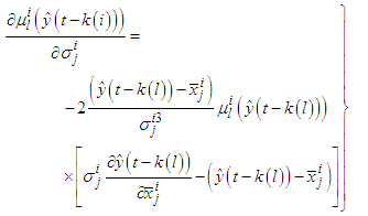
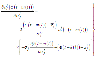
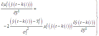 | (C-9) |
 | (C-10) |
 | (C-11) |
 | (C-12) |
 | (C-13) |
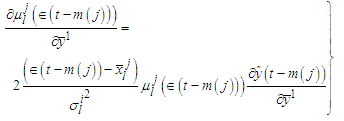
 represents all the adjustable parameter in the model excluding the consequences, and
 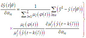 | (C-14) |
 is a parameter of the membership function
  and U is the set of rules that include in the antecedents the membership function
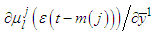
  . According to the type of membership functions and the regressors the term
 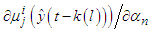 will have expressions, which are presented in the following lines. C.3.1. Gradient for the parameters of the Membership Functions with Gaussian Membership Functions With Gaussian membership functions
  could be
  and the gradients will be:
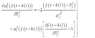 | (C-15) |
 | (C-16) |
 | (C-17) |
 | (C-18) |
 could be
  and the gradients will be
 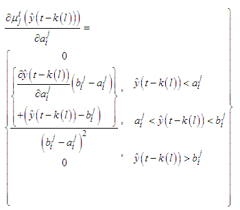 | (C-19) |
 | (C-20) |
 | (C-21) |
 | (C-22) |
 | (C-23) |
 | (C-24) |
 | (C-25) |
 | (C-26) |
 parameters could be
 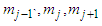 and the derivatives will be given by
 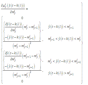 | (C-27) |
 | (C-28) |
 | (C-29) |
 | (C-30) |
 | (C-31) |
 | (C-32) |
 and the gradient expressions are reduced to the ones used for static functions. The presence of the terms
  in the gradients demands for computation of the gradients the calculation of a numerical solution of a discrete dynamic system, which must be updated each time a new data point is presented to the model.
Conflict of Interest
- The authors declare that they have no conflict of interest.