1. Introduction

Recently, the control problem of switched uncertain nonlinear systems has attracted much attention [1], [2]. For non-strict feedback uncertain switched nonlinear systems, an adaptive fuzzy output-feedback stabilization control method has been already studied in [1]. The adaptive fuzzy control problem of nonlinear switched stochastic pure feedback systems has been discussed in Yin et al. [2]. Also, a lot of decentralized controller design methods for switched nonlinear systems have been investigated and various successful control applications have been developed. Meanwhile, many research results of strict feedback form systems or non-strict feedback form systems have been proposed [3], [4]. In [3], an adaptive fuzzy controller has been presented for a class of switched uncertain nonlinear systems with strict-feedback form. Liu et al. [4] focus on backstepping-based adaptive neural control for switched nonlinear systems in nonstrict-feedback form.

Input saturation often occurs in practical engineering, which is a source of limiting the system performance severely and even leads to the system instability. Recently, the problem of input saturation has attracted much attention. Zhou et al. [5] presents an adaptive fuzzy control approach for a class of uncertain non-strict feedback systems with input saturation and output constraint. In [6], a fuzzy backstepping output tracking control approach was developed for a class of single-input-single-output (SISO) strict feedback nonlinear systems with unmeasured states and input saturation.

Sliding mode controller (SMC) is a powerful technique that has been successfully applied to control nonlinear systems with external disturbances and parameter variations. The SMC as ordinary design tools for control systems have been well accepted, and the major benefits of the SMC are the following: 1) its robustness against for a class of system uncertainties or perturbations; 2) a fast response and a good transient performance. Based on the aforementioned advantages, sliding mode control has been applied widely [7-9]. In [8], adaptive sliding mode approach was presented to handle disturbances of unknown bounds in nonlinear systems. Zhang et al. [9] proposed the sliding mode controller to tackle the trajectory tracking problems for discrete non-affine nonlinear systems with disturbance.

Fuzzy logic systems (FLSs) are employed to approximate the unknown nonlinear functions. Based on the universal approximation theorem, some stable adaptive fuzzy control schemes have been developed [10-12, 16-17] to overcome the difficulty of extracting linguistic control rule from experts and to cope with the system parameter changes. Zhao et al. [10] introduced an adaptive fuzzy hierarchical sliding mode controller to treat the problem for a class of multi-input multi-output unknown nonlinear time-delay systems with input saturation By means of two effective technical measures, more relaxed designs of discrete-time Takagi–Sugeno fuzzy-model-based observers was presented in [12]. The observer-based robust adaptive fuzzy control for MIMO nonlinear uncertain systems with delayed output has been discussed in [16]. Hwang et al. [17] presented an adaptive fuzzy hierarchical sliding-mode control for the trajectory tracking of uncertain under-actuated nonlinear dynamic systems.

In this paper, a fuzzy sliding mode control approach based on an observer is presented for a class of switched nonlinear systems with input saturation. Comparing with the existing results, the main features and contributions of this paper can be listed below.

(i) Based on the adaptive fuzzy control method, input saturation is considered in the design procedure, which is more common for application in practical engineering.

(ii) By sliding mode control technique design, an adaptive fuzzy sliding mode controller is designed for the system via using fuzzy logic systems to approximate uncertain functions, and the fuzzy state observer is employed to estimate the unavailable state for measurement.

(iii) Choosing an appropriate Lyapunov function, it is theoretically guaranteed that all the signals in the closed-loop system are uniformly ultimately bounded and obtain good system performance under our designed controller.

The remainder of this paper is organized as follows. Section II describes the problem formulation and preliminaries together with the definition of fuzzy logic systems (FLSs) are given. In Section III, adaptive fuzzy sliding mode controller and observer are designed for a class of switched uncertain nonlinear systems with input saturation and the stability analysis of the whole system is also verified by Lyapunov functional. Some computer simulation results of a practical example are indicated to show the performance of the proposed approach in Section IV. Finally, the conclusion is drawn in Section V.

2. Problem Statement and Preliminaries

2.1. System Description

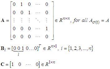
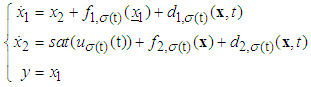
Consider a class of switched uncertain nonlinear systems with input saturation in strict-feedback from [15]:

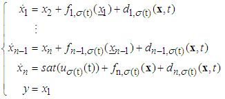(1)

where is the system state vector which is assumed to be unavailable for measurement, and are input and output of the system output, respectively. The function 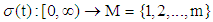, is a switching signal which is assumed to be a piecewise continuous (from the right) function of time. If , then we say the k-th switched subsystem is active and the remaining switched subsystems are inactive. 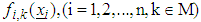are unknown smooth nonlinear functions, 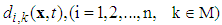are unknown external bound disturbances. denotes the nonlinear saturation characteristic.

Eq. (1) can be rewritten as

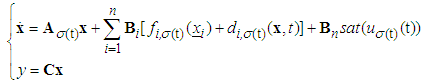(2)

where

Assumption 1: 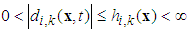, where are unknown functions.

In order to deal with the control constraints for convenience, the saturation function can be rewritten as

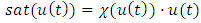(3)

where be expressed as

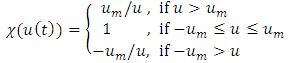(4)

Control Objective: Design a controller for (1) such that the states of the system will converge asymptotically to a neighborhood of zero.

2.2. Description of Fuzzy Logic Systems

The fuzzy logic system performs a mapping from to . Let where , . The fuzzy rule base consists of a collection of fuzzy IF-THEN rules:

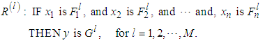(5)

in which and are the input and output of the fuzzy logic system, and are fuzzy sets in and , respectively. The fuzzifier maps a crisp point into a fuzzy set in . The fuzzy inference engine performs a mapping from fuzzy sets in to fuzzy sets in , based upon the fuzzy IF-THEN rules in the fuzzy rule base and the compositional rule of inference. The defuzzifier maps a fuzzy set in to a crisp point in .

The fuzzy systems with center-average defuzzifier, product inference and singleton fuzzifier are of the following form:

(6)

where with each variable as the point at which the fuzzy membership function of achieves the maximum value and with each variable as the fuzzy basis function defined as

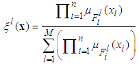(7)

where is the membership function of the fuzzy set.

3. Controller Design and Stability Analysis

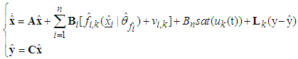
3.1. Observer Design

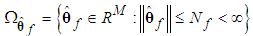
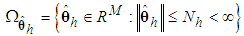
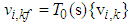
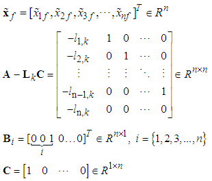
First, let the unknown nonlinear functions can be approximated over a compact set , by the fuzzy logic systems as follows:

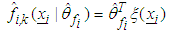(8)

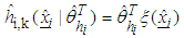(9)

where is the fuzzy basis vector, are the corresponding adjustable parameter vectors of each fuzzy logic systems.

Owing to the unavailable states of the system and the unavailable elements of the output error vector in many practical systems, the fuzzy logic systems (8) and (9) are not used to control nonlinear systems whose states are not obtained for measurement. Therefore, we must employ an observer to estimate. Let be defined as the estimates of . Then, we can obtain the following fuzzy logic systems as

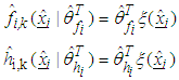(10)

In order to estimate the state, the observer for system (2) can be chosen as follows:

(11)

where, .

is the observer gain matrix to guarantee the characteristic polynomial of to be Hurwitz. Let us define the estimation error vector as and, then by (2) and (11), we obtain

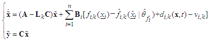(12)

It is assumed that belong to compact sets respectively, which is defined as

(13)

(14)

(15)

(16)

where are the designed parameters, and M is the number of fuzzy inference rules. Let us define the optimal parameter vector and as follows:

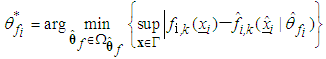(17)

(18)

where and are bounded in the suitable closed set and , respectively.

The parameter estimation errors can be defined as

(19)

(20)

(21)

(22)

are the minimum approximation errors, which correspond to approximation errors obtained when optimal parameters are used.

Applying (19) and (21), we obtain

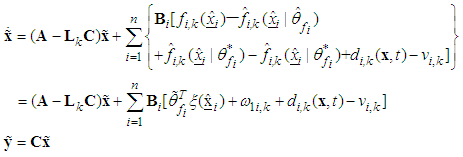(23)

The output error dynamics of (23) can be expressed as follows:

(24)

where

(25)

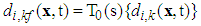
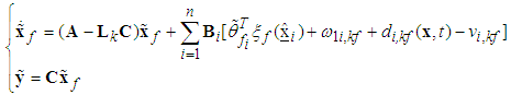
and s denotes the complex Laplace transform variable. As has been discussed, we could not obtain all elements of , because not all states of the system are available for measurement. Hence, we could not obtain all elements of . We will employ the state variable filters [14] to cope with this problem. First, we choose a stable filter as the following form:

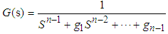(26)

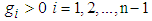where are coefficients of the Hurwitz polynomial.

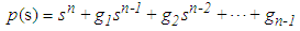(27)

Introducing (26) into (24), we can obtain the steady-state equation

(28)

Define a set of state variable filters

The corresponding filtered signals are defined as follows:

(29)

(30)

(31)

(32)

and

(33)

Then, Eq. (23) can be rewritten as follows:

(34)

where

Then, we define

(35)

and

(36)

where and are the estimated of and , respectively. The following assumptions are satisfied

(37)

(38)

Based on Lyapunov stable theorem, we can obtain the robust compensation term and the parameter update laws as follows:

(39)

(40)

(41)

(42)

(43)

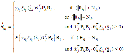
where and are positive constants.

Remark 1: Without loss of generality, the adaptive laws used in this paper are assumed that the parameter vectors are within the constraint sets or on the boundaries of the constraint sets but moving toward the inside of the constraint sets. If the parameter vectors are on the boundaries of the constraint sets but moving toward the outside of the constraint sets, we have to use the projection algorithm to modify the adaptive laws such that the parameter vectors will remain inside of the constraint sets. Readers can refer to reference [13]. The proposed adaptive law (40)-(43) can be modified as the following form:

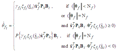(44)

where is defined as

(45)

(46)

where is defined as

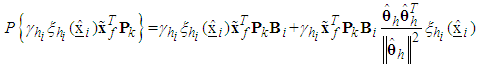(47)

The main result of robust adaptive fuzzy observer scheme is summarized on the following theorem.

Theorem 1: Consider a class of switched uncertain nonlinear systems with input saturation in strict-feedback from (1). The robust adaptive fuzzy observer is defined by (11) with adaptation laws given by (40)-(43). For the given positive definite matrix , if there exist symmetric positive definite matrix such that the following Lyapunov equation

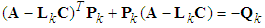(48)

is satisfied, then all the closed-loop signals are bound, and the estimation errors converge to a neighborhood of zero.

Proof. Consider the Lyapunov function candidate

(49)

(50)

By the time derivate of and the facts we obtain

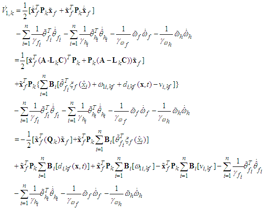From Assumption 1, it yields

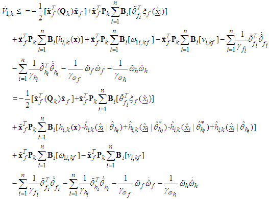By employing (20) and (22), we can get

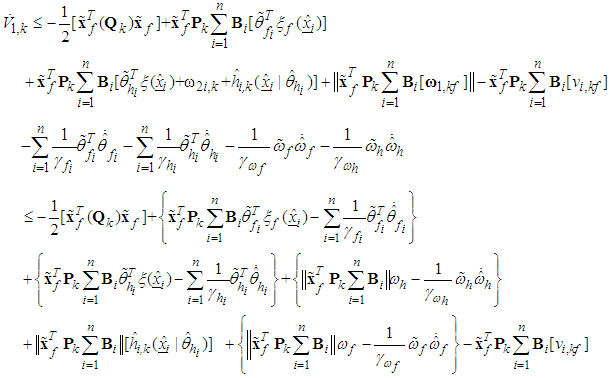(51)

Using (40)-(43), we have

(52)

Then employing the robust compensation term (39), the above equation can be rewritten as

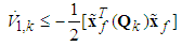(53)

Therefore, it can be concluded that from (53), and the estimation errors of the closed-loop system converges asymptotically to a neighborhood of zero based on Lyapunov synthesis approach. This completes the proof.

3.2. Controller Design

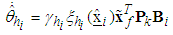
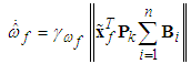
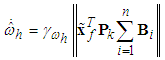
Next, we design the observer-based incremental sliding mode controller. Define the sliding surfaces as follows:

(54)

where for i=1, 2,…, n-1, are positive constants.

Differentiating with respect to time, we have

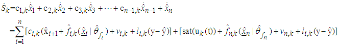(55)

The following controller can be chosen as:

(56)

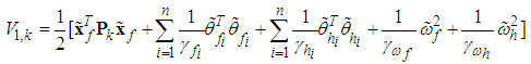
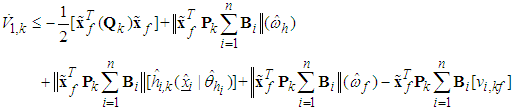
where can be obtained by backward from and is a positive constant.

Theorem 2: Consider the switched uncertain nonlinear system (1). The proposed adaptive fuzzy sliding mode controller defined by (56) with adaptive laws (40)-(43) guarantees that all signals of the closed-loop system are bounded, and converge to a neighborhood of zero.

Proof: Consider the Lyapunov function candidate . Differentiating the and with respect to time, we can obtain

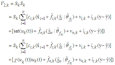(57)

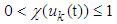Since according to the density property of a real number [7].

(58)

Then substituting equivalent control into (56), we have

(59)

Therefore, it can be concluded that from (59), and the all signals of the closed-loop system converges asymptotically to a neighborhood of zero based on Lyapunov synpaper approach. This completes the proof.

4. An Example and Simulation Results

In this section, a series of simulation results of a switched RLC circuit [15] as depicted in Fig. 1, described by

(60)

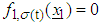where the nonlinear functions , , and for each denotes the k-th capacitor, denotes the charge in the capacitor and the flux in the inductance, respectively, and denotes the voltage. In the simulation, parameters of the RLC circuit are . The disturbances are assumed to be 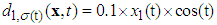and for .

In the implementation, five fuzzy sets are defined over interval [-2, 2] for with labels and their membership functions are

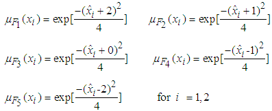
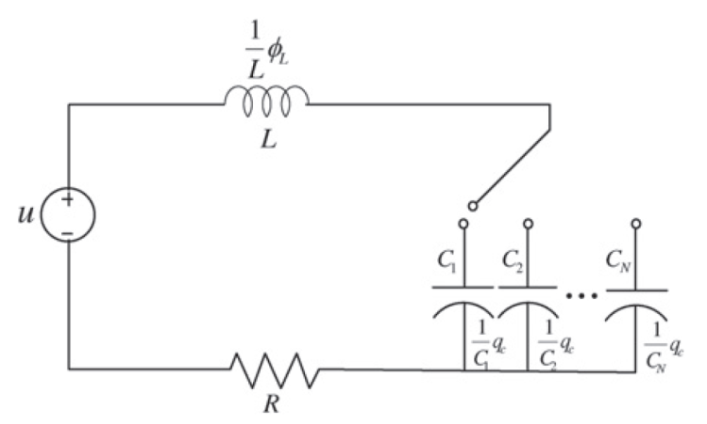Figure 1. The mass-spring-damper system

In this section, we apply the adaptive fuzzy robust observer-based sliding mode control approach in Section 3 to deal with the control problem. First, we select the observer gain as . The sample time is 0.01s. The sliding surfaces are selected as 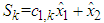when k = 1, 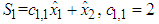and when k = 2, 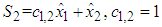. The initial values are chosen as

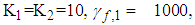
The other parameters are selected as . The simulation results are shown in Figs.2-11. Fig.2 and Fig.3 show the trajectories of the system states and their estimation states and Fig.4-5 show the trajectories of the system states estimation error. Figs.6 shows the phase plane plot of the system states Figs.7 demonstrate the trajectories of the system functions. Figs.8 shows the switch signal of the system. The performance of sliding surface and the control signal are shown in Figs.9-10 and Fig.11, respectively.

Figure 2. Trajectories of

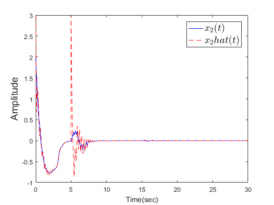Figure 3. Trajectories of

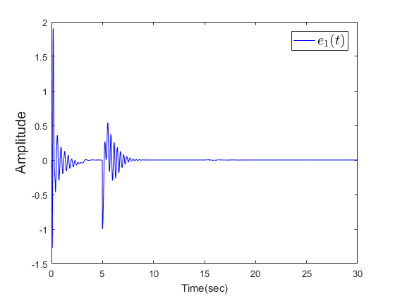Figure 4. The estimation error of

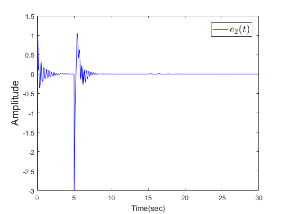Figure 5. The estimation error of

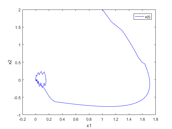Figure 6. Phase plane plot of the system states

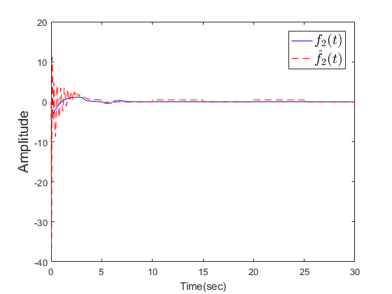Figure 7. Trajectories of

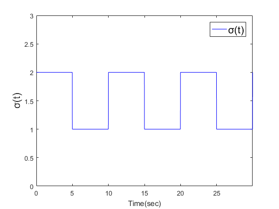Figure 8. Switch signal of the system

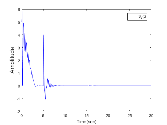Figure 9. The sliding surface

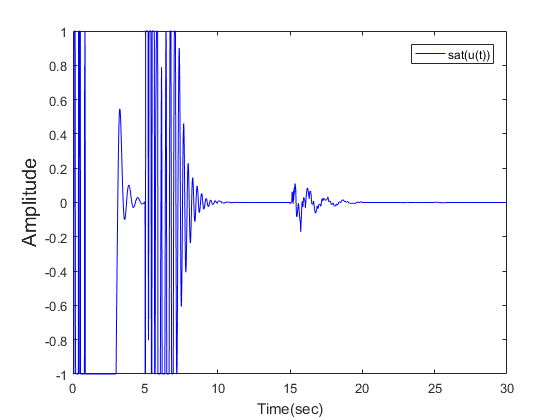Figure 10. Control signal with input saturation

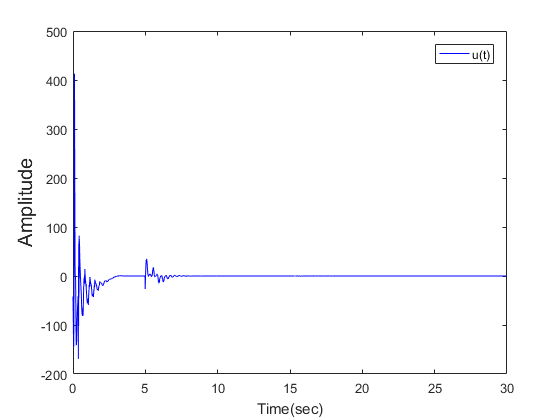Figure 11. Original control signal

5. Conclusions

An adaptive fuzzy observer-based sliding mode control approach has been proposed for a class of switched uncertain nonlinear systems with input saturation in strict-feedback form. A fuzzy state observer has been designed for estimating the unmeasured states with the help of FLS approximating the unknown functions. Based on the designed sliding mode controller, it can ensure the boundedness of the proposed sliding surfaces, which realizes the stability of system. By choosing an appropriate Lyapunov function, the proposed controller is designed to demonstrate that all the signals in the closed-loop system can not only guarantee uniformly ultimately bounded, but also achieve good performance. Finally, some computer simulation results of a practical example are illustrated to show the performance of the proposed control approach.