1. Introduction

Interpolation of functions is one of the most desirable methods of mathematical analysis. The main problem of function interpolation can be formulated as follows. It is given a finite set of couples¹

where I is a finite set of indexes. The problem is to construct a function,

Here is the given interval of the variable on which the interpolation is required. Naturally, Depending on the specific problem under consideration, can be bounded or unbounded.

Applications of the function interpolation ranges from numerical solution of ordinary and partial differential equations to solution of the best fitting problem for finite sets of data. Usually, real-life observations or measurements at discrete time-instants are gathered in a data set like For example, in astronomical observations of a planetary motion, are the time-instants when the coordinate of the center of mass of a planet is measured. In bio-laboratory, maybe the state of a mouse at time-instant The radiation intensity is measured at discrete points Finally, in particle tracing experiments, may be the coordinate of a particle observed at the time-instant In all those examples, it is a very important and challenging problem to know the measuring quantity at all (even non-measured) time-instants. This problem is usually solved by the methods of function interpolation theory [1-3].

2. Methods of Interpolation

The theory of function interpolation suggests a variety of methods to tackle such problems. The main tool of function interpolation is the construction of appropriate interpolating polynomials. There exists a handful of interpolating polynomials used in real-life applications. The most known interpolation types are piecewise constant interpolation, linear interpolation, polynomial interpolation, spline interpolation, rational interpolation, Padé approximant, Whittaker-Shannon interpolation (when is infinite), Hermite interpolation (when both the values of a function and its derivatives are given), wavelets, Gaussian processes (when the interpolating data contain some noise), etc. The choice of a specific interpolating method depends on such criteria as interpolation accuracy, low cost computer realization, ability to cover sparse data sets, etc.

The most delicate analysis require large and sparse data sets. For instance, in the case of large data sets, in order to perform a delicate analysis, the interval must be split into a large number of sub-intervals where the data (observations, measurements, etc.) are easier to interpolate. Then, interpolating functions are interpolated in each sub-interval and eventually the unknown function is represented as the totality of sub-interpolants. In other words, let

be a splitting of the set i.e,

and let be the corresponding interpolants, i.e.,

Then, the unknown function on the whole is defined as follows:

Here is a finite set of indexes. The choice of is conditioned by the choice of the splitting If contains only several points, then the simple interpolation tools such as piecewise constant or linear interpolation can be used efficiently. Schematic representation of the above mentioned is brought in Fig 1.

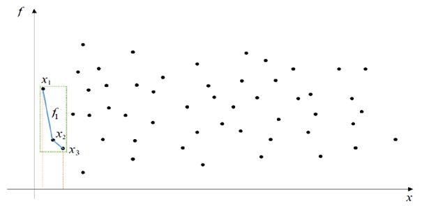Figure 1. Schematic representation of function interpolation over a large data set. Bold points represent the set Dashed lines draw the boundary of the first splitting consisting of Piecewise constant (linear) interpolation is used to construct . All other interpolating functions are constructed similarly

Remark 1 If the large data set under study is very dense, this approach may lead to enormous computational costs when numerically evaluating the interpolating function f. Contrary, if the large data set under study is sparse, the splitting gives a very efficient strategy. Thus, this approach is valid while the splitting provides a numerically efficient strategy.

Remark 2 Dense data sets are normally formed by the measurements of the very frequent processes or quantitates that changes over coordinate very rapidly. For a greedy algorithm based dense data analysis see, for instance [4].

Let us now describe some methods of function interpolation. One of the simplest methods of function interpolation is the linear interpolation. This method is valid when the set consists of only two couples. In such cases, the interpolating function is given as follows:

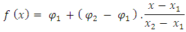Sometimes, piecewise constant (linear) interpolation is combined with the splitting method above to construct a linear interpolating function within each interval of splitting:

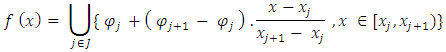In the case of regularly distributed points, polynomial interpolation is usually used. The most common polynomial interpolating functions are:

1. Lagrange interpolating polynomial:

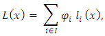Where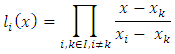

2. Newton interpolating polynomial:

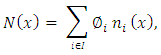Where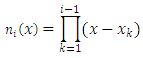

is the ith divided difference;

3. Chebyshev interpolating polynomials of the first and second kinds:

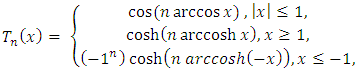
In the case of very dense data sets, the spline interpolation is more proffered than polynomial interpolation. As it is well-known, splines are defined piecewise in terms of polynomials of required order:

Thus, instead of piecewise constant (linear) interpolating functions, splines provide polynomial interpolation within each sub-interval of the splitting.

In the case of periodic or almost periodic data, such as tidal or climate change observation, trigonometric polynomials are used:

3. Artificial Neural Networks and Function Interpolation

Artificial neural networks possessing the ability of trained analysis and prediction may be especially advantageous in function interpolation. There exists several algorithms for constructing interpolation of a function by means of artificial neural networks. See, for instance, [5-18] and the related references therein for relevant studies.

The interest towards function interpolation by means of artificial neural networks increased during recent years is conditioned by the advantage shown in the numerical procedure of constructing the interpolating function. Due to the ability of prediction, neural networks allow to consider much less nodes than any other method of interpolation. Thus, solving the same problem requiring a much less computational time and resources. The numerical analysis carried out in the next section shows that it provides a better approximation of two special functions compared with the Lagrange interpolating polynomials with 50 and 100 nodes, respectively.

4. Comparison of Lagrange Interpolating Polynomial and Artificial Neural Network Interpolation

In this section we carry out a numerical comparison between interpolation of some well-known specific functions by means of the Lagrange interpolating polynomial and artificial neural networks.

First, let us consider the rectangular function defined according to the piecewise rule

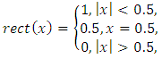Rectangular function has many applications in electrical engineering and signal processing. Besides, it serves as an activation function for many advanced neural networks.

The rect function also can be expressed in terms of the Heaviside function as follows:

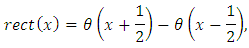Or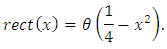

Let us remind that the Heaviside function is defined as follows:

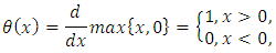Figures 2-4 show the numerical comparison of the interpolation of the rect function by means of Lagrange interpolating polynomial and artificial neural networks. Figure 3 shows that when we consider 50 nodes within , the quadratic error between the Lagrange interpolating polynomial and artificial neural network interpolation dramatically decreases up to 6th epochs. From 7th epoch on, the quadratic error remains almost unaltered and is of order.

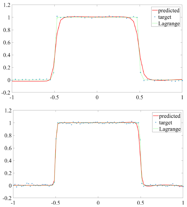Figure 2. Approximation of rect function in 50 nodes (upper) and 100 nodes (lower): ANN algorithm requires 10 and 15 iterations, respectively

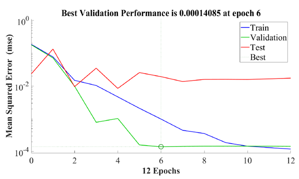Figure 3. Quadratic error approximation of rect function in with 100 nodes

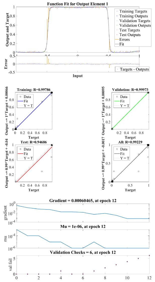Figure 4. Function fit (upper) and regression behaviour (middle) and network performance (lower) for rect function in with 100 nodes

We also show the advantage of the artificial neural network interpolation in the case of ramp function, defined as follows:

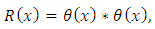where * denotes the convolution operation. Ramp function and has many applications in engineering (it is used in the so-called half-wave rectification, which is used to convert alternating current into direct current by allowing only positive voltages), artificial neural networks (it serves as an activation function), finance, statistics, fluid mechanics, etc.

According to the definition of the Heaviside function, the rump function can be represented also as

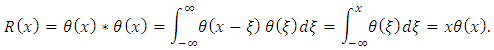The numerical comparison of the interpolation of the ramp function by means of Lagrange interpolating polynomial and artificial neural networks is shown in Figures 5-7. Figure 6 shows that when we consider 50 nodes within the quadratic error between the Lagrange interpolating polynomial and artificial neural network interpolation dramatically decreases up to 5th epochs. From 6th epoch on, the quadratic error remains almost unaltered and is of order.

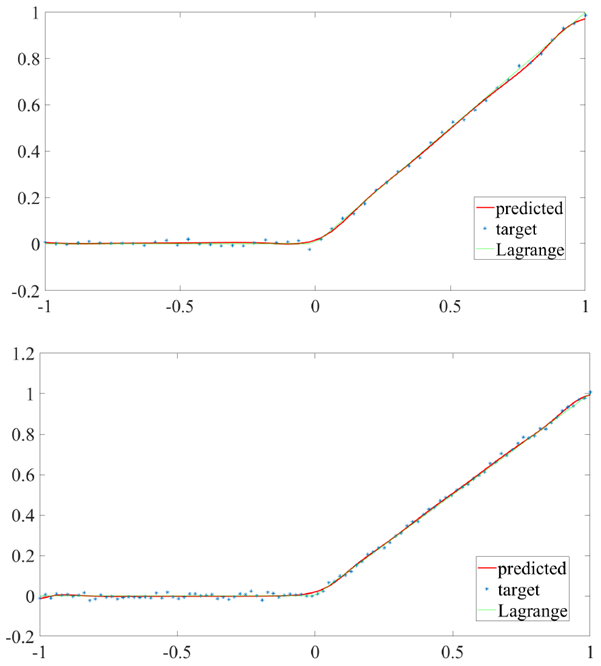Figure 5. Approximation of R function in with 50 nodes (upper) and 100 nodes (lower): ANN algorithm requires 15 and 29 iterations, respectively

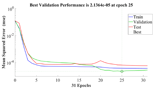Figure 6. Quadratic error approximation of R function in with 100 nodes

Figure 7. Function fit (upper) and regression behavior (middle) and network performance (lower) for R function in with 100 nodes

Finally, let us consider the triangular function defined as follows:

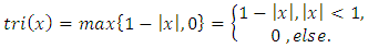On the other hand, the triangular function is defined as the convolution of the rectangular function with itself, i.e.,

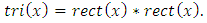Therefore,

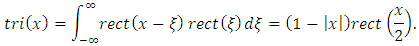Using the relation between the rectangular and Heaviside functions, it is possible to express the triangular function in terms of the Heaviside function. More specifically, since

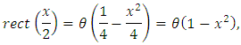by virtue of the trivial equality

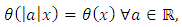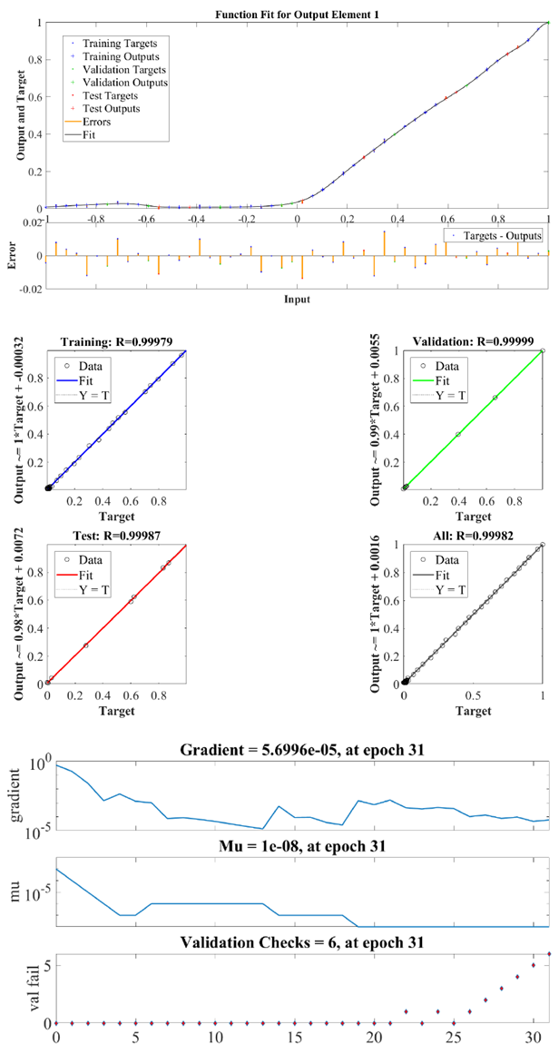
then

The numerical comparison of the interpolation of the tri function by means of Lagrange interpolating polynomial and artificial neural networks is shown in Figures 8-10. Figure 9 shows that when we consider 50 nodes within the quadratic error between the Lagrange interpolating polynomial and artificial neural network interpolation dramatically decreases up to 10th epochs. From 6th epoch on, the quadratic error remains almost unaltered and is of order.

Figure 8. Approximation of triangular function in with 50 nodes (upper) and 100 nodes (lower): ANN algorithm requires 12 and 30 iterations, respectively

Figure 9. Quadratic error approximation of triangular function in with 100 nodes

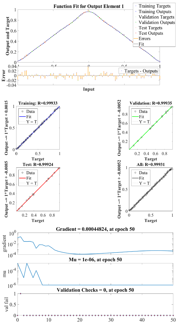Figure 10. Function fit (upper) and regression behavior (middle) and network performance (lower) for triangular function i with 100 nodes

5. Conclusions

In this paper we have studied the possibility of involving a computational neural network with a single hidden layer trained to interpolate functions with minimal number of nodes. The neural network is trained to start with the first several nodes and predict the proceeding nodes using the nearest-neighbour algorithm. The interpolation provided by the artificial neural networked has been compared numerically with the Lagrange interpolating polynomial. The algorithm is tested for the rectangular, ramp and triangular functions. It is observed that the quadratic error between the two interpolating methods dramatically decreases when the number of epochs is increased.

Notes

1. For the sake of simplicity, we restrict ourselves by the one-dimensional case. Higher dimensional (multivariate) cases are treated in the same way.

2. Again for the sake of simplicity we consider real-valued functions. Complex-valued functions can be considered similarly.