1. Introduction

With the Lehman Brothers bankruptcy filing, the largest in United States history, an economic crisis started in 2007 affecting the entire world. This catastrophic event has drawn the attention to the key role of the banks operating in the financial system that may cause a crisis. From the two large global crises that occurred in the last decade, it can be seen that the collapse of even one bank may cause a banking panic, thus widening the potential financial problem followed by a recession.

It is clear that bank runs and investment decisions are vital issues affecting global financial developments. Information of banking performance guides decision makers through the maze of financial planning therefore the prediction of bank failure such as classification of banks as successful or unsuccessful is a crucial issue.

Turkey suffered a major economic crisis in 2001 following the Asian crisis. Failures in the banking sector caused a dramatic financial collapse, affecting the economic system in the entire country. Nearly half of the Turkish banking system, 21 commercial banks, has been put under the control of the Saving Deposit Insurance Fund (SDIF) reflecting the failure of Turkish banks. This catastrophic economic situation awakened the authority for the need of the constant monitoring activity.

There are several academic studies that aim to discriminate between sound and weak banks. It is possible to distinguish the classification techniques that have been used for failure prediction as data mining techniques (Classification and Regression Trees, Neural Nets, K-Nearest Neighbor, Association Rules, Cluster Analysis) and classical statistical techniques (Regression, Logit/Probit, Duration Models, Principal Components, Discriminant Analysis, Bayes Rules). While classical methods focus on estimating the parameters under the assumption that the structure of the model is known, data mining techniques use an algorithmic paradigm, which assumes that the functional form of data is unknown.

Lately, with the rapid advancement of technology in all sectors, and especially in finance, databases are overflowing and the idea is gaining popularity that data should be analyzed with data mining techniques rather than the classical statistical methods, or with a combination of both artificial intelligence and statistical methods. One of these aggregation methods is support vector machines (SVMs), which use statistical thinking, optimization, and machine learning rules together. [1] applied t-tests to show the importance of the financial ratios for the discrimination between failed and surviving firms. [2, 3] extended the study using statistical techniques. [4] pioneered the researchers for the prediction of bank failure. To follow the extensions from the literature a researcher should refer to the reviews published by [5, 6], Hossari, (2009), [8, 9].

Following the big bankruptcy case of the banks in Turkey several bank-failure studies have been made focusing on the period between 1997 and 2001. These studies were mainly cross-sectional and were done by [10-15]. [16] have conducted a research about bank failures using a longitudinal data set. They implemented logistic regression, generalized estimating equations and marginalized transition models and concluded that all three models performed equally well.

This study aims to conduct a longitudinal data analysis about the financial ratios of Turkish commercial banks from for the period between 1994 and 2001 to predict bank failure using a multiplicative neuron model artificial neural network (MNM-ANN) that is trained using particle swarm optimization (PSO) and support vector machines (SVMs) with the radial basis kernel function.

Being taken over by SDIF is a useful failure definition for the banks and some other commercial entities. Thus, in this study, the seizure of the funds by the SDIF was accepted as a bank failure definition. To our knowledge there is no bank bankruptcy study using both longitudinal data and the methods applied here.

A review of modelling corporate collapse is given in Section 1. The second section discusses the theoretical backgrounds of the artificial intelligence models applied to the banks’ financial ratios. Section 3 details the application part. The results and findings are given in Section 4. Section 5 concludes, including the recommendations regarding future works.

2. Theoretical Background

2.1. Longitudinal Data

A long term data structure is considered in this study. Longitudinal data includes a cross-section of units observed over time and gives a chance to study dynamic relationships and heterogeneity.

Generally, when one uses longitudinal data for classification purposes, a fixed effect or random effect logistic regression model is used. These methods have the benefits of longitudinal data but encounter some problems, such as misspecification of the model structure or failure to meet the model assumptions. Data mining methods can be used to overcome the problems regarding such assumptions. There are several artificial intelligence methods used to classify successful and unsuccessful banks. We will apply a PSO-based MNM-ANN, and SVM models to a longitudinal bank bankruptcy data.

2.2. The Framework of Machine Learning Technique

In general, classification models are trained on previous results with known labels. These classifiers, once trained, can then be applied to predict the labels of new samples. ANN and SVMs are inductive machine learning techniques; therefore they are described in terms of machine learning framework.

We take be a set of training data of elements where is a vector of elements of an dot product space and as a sample set of this space [17]. Here stands for the number of the independent variables and the values of the variables are real numbers.

In binary classification problems, data is to be labelled +1 or -1. The goal is to develop a model to predict the original tagging function when y is the dependent, or class, variable. This is done by constructing a hyperplane which provides an optimal separation between the +1 and -1 classes. This linear decision surface can be used to as the basis for the model The linear decision surface is written as where is the points’ position vector and is the surface’s normal vector. will define a line in two-dimensions, a plane in three-dimensions and so on.

2.3. Multiplicative Neuron Model Artificial Neural Network

Artificial neural networks are free of the assumptions such as linearity and normality; therefore, they have been widely used for prediction and classification purposes for years.

Generally, an artificial neural network uses hidden layers and a summation aggregation function. In this study we applied a MNM-ANN, which has a multiplicative aggregation function to our longitudinal data.

[18] were the first to introduce MNM-ANN, which uses only one multiplicative neuron in the hidden layer, for time series prediction. Since MNM-ANN has one neuron, the problem about determination of the number of hidden layer neurons, which is naturally problematic, is naturally solved. The present method, which has no such limitation, is thus very advantageous in comparison. In their study, the architecture of MNM-ANN was defined as in Fig. 1. are inputs of MNM-ANN.

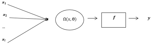Figure 1. Structure of MNM-ANN

As it is seen from the architecture MNM-ANN has a multiplicative structure with an aggregation function of . The output of this single neuron is calculated as shown below:

(1)

where are weight and bias vectors corresponding to the i^th input for . [18] selected logistic function as the activation function (𝑓). One can calculate the output of MNM-ANN as the labels either +1 or -1 using logistic activation function as follows:

(2)

2.4. Training MNM-ANN Using PSO

The observed data of input and output values are used to find a set of weights and bias values so that the neural network generates estimated outputs that closely match the known outputs. This process is called training the neural network.

Different training approaches can be used in order to train a neural network. Among those algorithms the most popular methods are the error backpropagation and the Levenberg-Marquardt algorithms. In this study we have used a particle swarm optimization (PSO) based training technique to train single MNM-ANN.

Similar to genetic algorithm, particle swarm is a computational intelligence technique based on population behaviour. It was inspired by social behaviour and pioneered by [19]. Collection of individuals, same as a flock of birds, called particles move in steps throughout a region. It starts with a candidate solution and gradually evaluating the objective function at each step for each particle, it decides on the new velocity of each particle. The particles move using the simple mathematical formulae regarding the particle’s velocity and position. The algorithm re-evaluates until to the best solution.

The basic PSO algorithm for a group of i particles moving in an n-dimensional search space can be given as below:

Step 1. Randomly generate the position and the velocity for the i^th (i=1, 2, ..., p_n) particle, where n is the particle number.

Step 2. Compute the particle’s fitness value for every individual particle.

Step 3. Evaluate p_best and g_best according to the evaluation function. If the value of fitness corresponding to gbest is smaller than or if the maximum number of iterations is reached, tuning will stop. Otherwise continue with Step 4.

Step 4. Update the position and velocity for each particle using (3) and (4).

(3)

(4)

In the equation (3) is called as the inertia parameter that keeps the swarm together and prevents it from diversifying excessively. The acceleration factors are cognitive and social coefficients that control the impact of personal and common knowledge, respectively. A uniform distribution is used to generate the independent random numbers and is the best individual position for particle i, and stands for the best position reached by the group in the j-th axis. represents the j-th velocity value of the i-th particle; is the corresponding position of the particle. k is the current iteration number.

In literature it has been shown that varying inertia parameter and cognitive and social coefficients over the course of the optimization can have positive impacts on the results. In their study, [20] changed the cognitive and social coefficients during the iterations using the formulations (5) and (6).

(5)

(6)

(7)

If the inertia parameter and cognitive and social coefficients have been changed according to (5), (6), and (7) during the iterations, the new algorithm is called a modified particle swarm optimization algorithm. Once the network has been trained with data at hand and weights are obtained for each node, it can be used in order to predict a class label regarding the future.

2.5. Support Vector Machines using Gaussian Radial Basis Kernel Function

In recent studies, the use of artificial intelligence has become prevalent. Many studies have shown that artificial intelligence methods, such as neural network methods and support vector machines, can perform better than traditional statistical methods. Some researchers such as [21] indicated that there are several drawbacks in building a neural network model, such as the difficulty of determining the controlling parameters and the convergence of a local minimum solution instead of a global solution. As Shin et al. stated, that it is possible to find a solution that fits the training set but does not exhibit good performance for the test set. For good classification and prediction performance another challenge is to determine the size of the training set.

Difficulties encountered in the implementation of neural networks led to the development of a statistical learning method called support vector machines which are originally attributed to [22]. SVMs can be used for small sample sizes and large independent variables. They are less susceptible to overfitting, use structural risk minimization and are considered as a promising classifier by several researchers.

The goal in support vector machines approach is to find a separating linear decision surface located at equal distances from class boundaries. In the solution phase, the distance between class boundaries is also maximized. This distance which is tried to be maximized is called margin. When the problem is addressed in this way, the possibility of misclassification is reduced. The position of the decision surface is determined by the support vectors located on the supporting surfaces. These support vectors are the training set points with the heaviest constraints on the solution.

Constructing a maximum-margin classifier that maximizes the margin between the two supporting hyperplanes is indeed a convex optimization problem in the feasible solutions are all possible decision surfaces with their associated supporting hyperplanes, and can be solved via quadratic programming techniques.

Many complex learning algorithms have free parameters that must be estimated via experimentation with the training set. Consider the optimal topology in artificial neural networks or the optimal pruning constant in decision tree learning algorithms. A marked exception is the dual of the maximum-margin algorithm that is considered to construct a maximum-margin classifier without free parameters. This dual algorithm is called a linear support vector machine [17].

To define the maximum margin classifier, assume that a linearly separable training set is given the form . Then the primal maximum margin optimization problem is formed so as to maximize the margin as:

(8)

where is the margin of the optimal decision surface

Using the duality concept, (8) can be converted to a minimization problem:

This objective function is subject to the constraints expressed in (9) and (10). All training points are used to define the feasible region:

(9)

(10)

The constraints can be rewritten in the form of a Lagrangian objective function which is constructed as:

(11)

Therefore the Lagrangian optimization problem for SVM is built as,

Subject to,

for

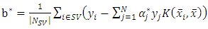
Because the objective function is a convex function, a maximum-margin decision surface can be computed using a quadratic programming approach that solves the generalized optimization problem. However, when actually computing such maximum-margin classifiers using quadratic program solvers, it has been found that the solutions depend heavily on how the free offset term parameter b has been chosen. It is possible to avoid this problem using the concept of duality.

The dual is obtained as:

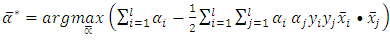(12)

Subject to the constraints

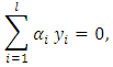
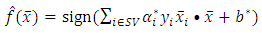
for This implies that the classification problem can be solved using linear support vector machine as long as the classes are linearly separable. After solving the quadratic optimization problem, the optimal dividing hyperplane is computed as:

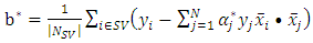
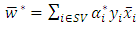(13)

and the offset term of the hyperplane is computed as:

(14)

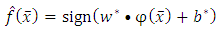
Respectively, where is the list of the training vectors, and are their respective labels, are the Lagrangian coefficients and SV is a set of support vectors. As a result, and can be used to classify the observations using the decision function given as:

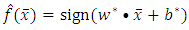(15)

In terms of dual representation the decision function can be rewritten as:

(16)

Remarkably, if we choose these transformations carefully, all the computations associated with the feature space can be performed in the input space. That is, even though we are transforming our input space so that the data become linearly separable, we do not have to pay the computational cost for these transformations.

The functions associated with these transformations are called kernel functions, and the process of using these functions to move from a linear to a nonlinear support vector machine is called the kernel trick. The trick lies in finding the appropriate kernel in order to construct a model for a particular data set.

When the data is linearly separable, a separating hyperplane may be used to divide the data. However, in the real world it is hard to find a case in which the data are linearly separable. In cases where date are not linearly separable, a transformation can be used to map the input data into a high-dimensional space called a feature space to make the data linearly separable.

Suppose that there is a mapping function that takes a point from the input space and maps it into the so-called future space F, considering that this new future space is linearly separable. Using the mapped data points instead of the decision function can be rewritten as:

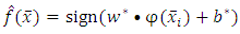(17)

where the natural inner product for Euclidean space is replaced with the natural inner product in the future space

(18)

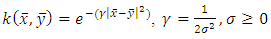
The trick part of the kernel trick appears with a kernel function as a positive semi-definite matrix that computes the inner product between any two finite sequences of inputs as a similarity measure and is defined as Therefore all the dot products in equations (8) and (12) can be replaced with Therefore and become:

(19)

(20)

and the classification rule looks like:

(21)

The very important part of SVMs is to find the appropriate kernel in order to construct a model for a particular data set. There are several proposed kernel functions in literature. The three most common kernel functions used for SVM are polynomial, Gaussian, and sigmoid functions [23].

For complex decision surfaces, Gaussian kernels have been used widely because they allow the data to be mapped onto an infinite-dimensional space [24] and they are defined as:

(22)

In the application part of this study, a Gaussian kernel will be used.

3. Implementation and Results

3.1. Implementation

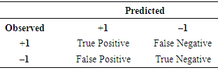
This study used SVMs with radial basis functions (RBFs) and Multiplicative Neuron Model Artificial Neural Network (MNM-ANN) trained using Particular Swarm Optimization (PSO) to classify Turkish commercial banks as failed or non-failed. MNM-ANN is offered as a promising technique for classification purposes but has not been used for bank failure studies yet. SVMs have been used for the purpose of bank classification in a few studies [14] but have not been applied to longitudinal data structures to our knowledge. RBFs were used as kernel functions to compute the inner products of the data to transform the data into a high-dimensional feature space. Financial ratios were studied to reveal their effect on bank performances.

The set of banks and the financial data required to train and test the MNM-ANN and SVMs were obtained from an official website, which provides financial tables and overall performance data of the Turkish finance sector. (http://www.tbb.org.tr/english/).

There are a total of 55 unsuccessful and 224 successful banks in the longitudinal data set for the 1994–2000 time period. For the banking status and a dependent variable according to the ownership, the code 1 is assigned to failed banks and 0 is assigned to successful banks. The banks controlled by the Saving Deposit Insurance Fund (SDIF) were defined as “failed,” and the rest were defined as “successful.”

The financial indicators (ratios regarding liquidity, profitability, efficiency, solvency, and leverage) from the annual reports of the banks are used as independent variables. For a complete list of these banks and financial ratios one can refer to [14].

There are plenty of financial ratios that may point out banks’ performance, and some of these ratios are highly correlated with one another. Therefore in this study we first have excluded financial ratios with correlations higher than 0.90. Then we have used factor analysis to construct independent factors that affect the success status of the banks. We have found that 18 financial ratios are appropriate for factor analysis.

Because the data are in longitudinal form, we have used the Levin-Lin-Chu unit root test to check whether the financial ratios are stationary. It is found that all ratios are stationary and appropriate for classical factor analysis.

Seven factors were found meaningful according to the eigenvalue criteria, chosen as being greater than one. meaningful factors are: Interest income and expenditures, equity, other income and expenditures, balance sheet, deposit, due, and asset quality.

The longitudinal data has been split into three different subsets, 90/80/70 percent for training and 10/20/30 percent for testing. Each of the three cases was trained and tested five times and the means were calculated. Stata 12 and Matlab R2011b were to process the data.

To assess the models, both MNM-ANN and SVMs were trained using the training data set and then they were tested using the new data sets. The results of the models were appraised using both ROC (Receiver Operating Characteristic) curves and a confusion matrix. The area under the ROC curves measures discrimination, that is, the ability of the models to correctly classify those banks with and without failure.

As with any classification problem, four outcomes can be represented in a confusion matrix given in Table 1. The confusion matrix then gives several metrics of a model’s performance. Correct classification rate (CCR), which is typically taken to be the most important performance metric, is the fraction of correctly predicted banks performances from the whole set of the banks. Sensitivity (Sen) is another straight-forward metric for the performance of a given model. It is defined as True Positive divided by the sum of all of the actual positives. Sensitivity measures how good a model is able to find positive results. And in certain situations such as failed banks, sensitivity can be seen as more significant than the accuracy. On the other hand if someone is interested in finding negative instances Specificity (Spe) can be used as the most important measure; specificity can be computed dividing True Negative by the total of all negatives.

Table 1. The results for the train/test set

3.2. Results

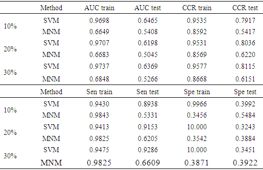
Considering the effects on the financial system, it is more important to identify a bank that is at risk of bankruptcy than to detect a healthy bank correctly. Therefore sensitivity is used as a performance criterion in this study.

Beside the sensitivity, overall correct classification rate (CCR), area under curve (AUC) and specificity (Spe) were calculated for the trained models and for three different percentages of test set (10%, 20%, and 30%). The results are given in Table 2.

Table 2. The results for SVM and MNM for both the train and test set

When the area under curve is prioritized, it is seen that support vector machines (SVMs) performed remarkably better than MNM-ANN single multiplication. Based on correct classification rate, however, for both train and test sets, support vector machines performed better. Regarding sensitivity, it is noteworthy that when the rate for support vector machines does not change very much, from 94% to 89%, there is an important decrease, from 98% to 53% in the multiplicative neuron model for the ten-percent test data. This means that support vector machines are superior compared to MNM-ANN for finding an unhealthy bank. On the other hand with regarding specificity, it is worthy to note that when the rate for support vector machines decreases from 99% to 39%, there is an increase in the multiplicative neuron model from 34% to 54% for ten-percent test data. This means that the multiplicative neuron model is better at finding healthy banks. Finding an unhealthy bank is more important than detecting healthy banks, according to the sensitivity measure, as well as the correct classification rate and ROC area, radial-basis support vector machines perform better than the multiplicative neuron model artificial neural network method in classifying banks as healthy or unhealthy.

4. Conclusions

In this study, the multiplicative neuron model artificial neural network and support vector machines were used to analyze bank health based on financial ratios. MNM-ANN is based on particle swarm optimization and SVMs are based on radial bases kernel. Turkish commercial banks’ financial ratios were used for both training and test sets of the models.

According to the results obtained, both multiplicative neuron model and support vector machines are able to extract useful information from financial data. However, when the main objective was to find positive examples, i.e. failing banks, the best predictive performance was achieved, taking into account the longitudinal structure of the data, using radial basis kernel function based support vector machines.

Although we have presented that the radial basis function performed as well as the kernel function, developing a suitable data-based kernel for longitudinal data sets would be an important piece of work within this line of research.

ACKNOWLEDGEMENTS

The research for this article was supported as a D-Type project numbered as FEN-D-100615-0282 by Marmara University Scientific Research Projects Committee.