-
Paper Information
- Paper Submission
-
Journal Information
- About This Journal
- Editorial Board
- Current Issue
- Archive
- Author Guidelines
- Contact Us
American Journal of Intelligent Systems
p-ISSN: 2165-8978 e-ISSN: 2165-8994
2017; 7(1): 1-18
doi:10.5923/j.ajis.20170701.01

Neural Network-Based Adaptive Speed Controller Design for Electromechanical Systems (Part 2: Dynamic Modeling Using MLMA & Closed-Loop Simulations)
 Abstract
 Reference
 Full-Text PDF
 Full-text HTML
Vincent A. Akpan1, Michael T. Babalola2, Reginald A. O. Osakwe3
1Department of Physics Electronics, The Federal University of Technology, Akure, Nigeria
2Department of Physics Electronics, Afe Babalola University, Ado-Ekiti, Nigeria
3Department of Physics, The Federal University of Petroleum Resources, Effurun, Nigeria
Correspondence to: Vincent A. Akpan, Department of Physics Electronics, The Federal University of Technology, Akure, Nigeria.
| Email: |  |
Copyright © 2017 Scientific & Academic Publishing. All Rights Reserved.
This work is licensed under the Creative Commons Attribution International License (CC BY).
http://creativecommons.org/licenses/by/4.0/

The dynamic modeling of an electromechanical motor system (EMS) for different input voltages based on different weights and the corresponding output revolutions per minute using neural networks (NN) is presented in this paper with a view to quantify the effects of voltages based on different weights on the system output. The input–output data i.e. the electrical input voltage and the revolution per minute (rpm) of a PORCH PPWPM432 permanent magnet direct current (PMDC) motor as the output which is obtained from the EMS have been used for the development of a dynamic model of the EMS. This paper presents the formulation and application of an online modified Levenberg-Marquardt algorithm (MLMA) for the nonlinear model identification of the EMS. The performance of the proposed MLMA algorithm is compared with the so-called error back-propagation with momentum (EBPM) algorithm which is the modified version of the standard back-propagation algorithm for training NNs. The MLMA and the EBPM algorithms are validated by one-step and five-step ahead prediction methods. The performances of the two algorithms are assessed by using the Akaike’s method to estimate the final prediction error (AFPE) of the regularized criterion. The validation results show the superior performance of the proposed MLMA algorithm in terms of much smaller prediction errors when compared to the EBPM algorithm. Furthermore, the simulation results shows that the proposed techniques and algorithms can be adapted and deployed for modeling the dynamics of the EMS and the prediction of future behaviour of the EMS in real life scenarios. In addition, the dynamic modeling of the EMS in closed-loop with a discrete-time fixed parameter proportional-integral-derivative (PID) controller has been conducted using both networks trained with EBPM and the MLMA algorithms. The simulation results demonstrate the efficiency and reliability of the proposed dynamic modeling using MLMA and closed-loop PID control scheme. However, despite the little poor performance of the PID controller, the accuracy of the NN model trained with the MLMA when used in a dynamic operating environment has been confirmed.
Keywords: Artificial neural network (ANN), Dynamic modeling, Electromechanical motor systems (EMS), Error back-propagation with momentum (EBPM), Modified Levenberg-Marquardt algorithm (MLMA), Neural network nonlinear autoregressive moving average with exogenous inputs (NNARMAX), Nonlinear model identification, Proportional-integral-derivative (PID) control
Cite this paper: Vincent A. Akpan, Michael T. Babalola, Reginald A. O. Osakwe, Neural Network-Based Adaptive Speed Controller Design for Electromechanical Systems (Part 2: Dynamic Modeling Using MLMA & Closed-Loop Simulations), American Journal of Intelligent Systems, Vol. 7 No. 1, 2017, pp. 1-18. doi: 10.5923/j.ajis.20170701.01.
Article Outline
1. Introduction
- Adaptive control has been extensively investigated and developed in both theory and application during the past few decades and it is still a very active research field [1-15]. In the earlier stage, most studies in adaptive control concentrated on linear systems [15]. A remarkable development in adaptive control theory is the resolution of the so- called ideal problem, which is the proof that several adaptive control systems are globally stable under certain ideal conditions. Then the robustness issues of adaptive control with respect to non ideal conditions such as external disturbances and unmodeled dynamics were addressed which resulted in many different robust adaptive control algorithms [1, 2]. Adaptive control algorithms can be applied for the control of any nonlinear dynamic system. But a model of the system is required [3, 15] A recent approach to modeling nonlinear dynamical systems is the use of artificial neural networks (ANN) or simply neural networks (NN). The application of neural networks for model identification and adaptive control of dynamic systems have been studied extensively [3-14]. As demonstrated in [3, 7, 8, 10, 11, 15], neural networks can approximate any nonlinear function to an arbitrary high degree of accuracy. The adjustment of the NN parameters results in different shaped nonlinearities achieved through a gradient descent approach on an error function that measures the difference between the output of the NN and the output of the true system for given input data, output data or input-output data pairs (training data).The Adaptive speed control of electromechanical systems has been widely studied and performed using various methods and components in the design and experiments [16-18]. However, the speed control could be achieved with either adaptive or conventional non-adaptive control methods. In adaptive control, there exists a feedback control with the ability of adjusting its speed in a changing environment so as to satisfy or maintain a set or desired speed. The actual speed is kept by speed controller to follow reference speed command. Adaptive control algorithms can be classified as either direct or indirect, depending on whether they employ an explicit parameter estimation algorithm within the overall adaptive scheme. By updating the required modeling information, perhaps through closed-loop identification, a direct adaptive control algorithm can be converted to an indirect adaptive control algorithm, which may yield greater versatility in practice. While model reference adaptive controllers and self tuning regulators were introduced as different approaches, the only real difference between them is that model reference schemes are direct adaptive control schemes whereas self tuning regulators are indirect. The self tuning regulator first identifies the system parameters recursively, and then uses these estimates to update the controller parameters through some fixed transformation. The model reference adaptive schemes update the controller parameters directly (no explicit estimate or identification of the system parameters are made).Many intelligent control techniques [19], such as artificial neural network and adaptive fuzzy logic control (AFLC) methods, have been developed and applied to control the speed of permanent magnet direct current (d.c.) motor, in order to obtain high operating performance [20]. Moreover, the development of AFLCs can be used to cope with some important complex control problems such as stabilization and tracking system output signals, the presence of nonlinearity and disturbance. Adaptive control schemes are generally used to control systems which include unknown and time-varying parameters [21].The ultimate aim of this research is to develop an adaptive speed controller that will maintain a desired reference trajectory of 60 rpm despite disturbances and its effects on the electromechanical system. At the center of the electromechanical system is a permanent magnet d.c. (PMDC) motor. Generally, d.c. motors are one of the most widely prime movers in industries today. They play important roles in energy conversion processes where they convert electrical energy into mechanical energy. In mechanical systems, speed varies with the number of tasks. Thus, speed control is necessary to do mechanical work in a proper way. It makes the motor to operate easily [22]. The speed of d.c. motor is directly proportional to the supply voltage. The d.c. motor is the obvious proving ground for advanced control algorithms in electric drives due to the stable and straight forward characteristics associated with it. It is also ideally suited for trajectory control applications. From a control system point of view, the d.c. motor can be considered as single input single output (SISO) plant, thereby eliminating the complications associated with a multiple-input multiple-output (MIMO) systems [23, 24]. To control any system, the basic understanding of the system is required. We need to understand the input and output behaviour of such system which will allow for the control of the system. All the inputs of real systems are always actuated by control signals from the controller while the system outputs on the other hand are measured using a sensors. The speed control and optimization of electromechanical systems has become imperative due to its applications in real life scenarios, any improvement made in this regard will be a novel contribution.Some of the more commonly occurring electromechanical systems are presented using linear transfer functions within each and every block defining the systems. In real designs, nonlinear elements frequently occur. However, such nonlinear components cannot be approximated by linear differential equations with constant coefficients (e.g. the Laplace solution techniques) [25]. Therefore, this work focuses on the formulation of neural network-based modeling algorithm that will capture the nonlinear dynamics of the EMS where such model can be used for the development of adaptive control algorithm for the adaptive speed control of EMSs.The paper is organised as follows. The description of the EMS is presented in Section 2. An overview of the EMS design and construction as well as information on the technique of data acquisition from the EMS are also presented in this section. Section 3 presents the formulation of the neural network-based modified Levenberg-Marquardt algorithm (MLMA) for NNARMAX model identification. Three validation algorithms are also presented in this section. The dynamic modeling and closed-loop simulations with a PID controller together with the simulation results are given in Section 4. A brief conclusion and possible directions on future work is given in Section 5.
2. Description of the EMS
- This section presents an overview of the design and development of the EMS. The complete design and fabrication procedure for the system can be found in [26]. The measurement procedure with the description of the EMS input-output data that describes the system behaviour, the considerations of the electromechanical system and the effects of the process variables on the system are also detailed in [26].
2.1. Design of the EMS
- The actuator used in this project is a PORCHE PPWPM432 windshield wiper motor which has a worm gear and simple ring gear that gives the device its incredible torque. This type of motor is called a “gearhead” or "gear motor" and has the advantage of having lots of torque. The system has been designed to accommodate different standard weights which are to be loaded through the bowl fitted to the iron sheet plate with bolts and nuts to hold it firmly as it rotates. The sheet (46 cm diameter, 0.1 cm thickness) is welded to the motor system with a shaft connected to the motor through the gearing system which transfers the motion of the motor to the bowl. Bearings were fitted to allow for free movements or rotation of the system and balancing rods were clamped to hold the system from falling and to maintain balance while rotating. The light dependent resistor (LDR) sensor is installed and aligned with the light source to receive the incident light through the hole of 2.5 cm bored on the sheet. The following is a list and specification of materials used for the design of the proposed electromechanical motor system, namely: 1). a PORCHE PPWPM432 windshield wiper motor with 19.6 cm diameter; 2). a container bowl with 21 cm height, 18.8 cm bottom diameter and 30 cm top diameter; 3). an iron sheet plate of 46 cm diameter, 0.1 cm thickness with a 2.5 cm hole for the sensor; 4). two gears 45 teeth and 35 teeth with 4.5 cm diameter and 3.5 cm diameter respectively; and 5). an Iron shaft of 19.4 cm length and 5.1 cm diameter (please see [26] for more detail).The sensor and bulb are installed at the bottom and top respectively with 4.5 cm equidistant from the iron sheet plate. A well labelled schematic diagram of the proposed electromechanical motor system is shown in Fig. 1(a) and a well labelled 3-D diagram of the proposed electromechanical motor system is also shown in Fig. 1(b) for a 3D view of the system.
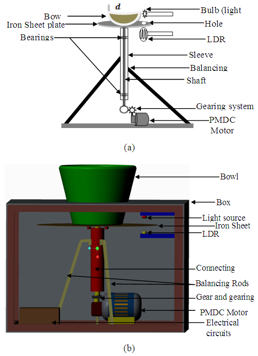 | Figure 1. The designed electromechanical motor system: (a) Schematic drawing of the electromechanical system and (b) 3-D drawing of the electromechanical speed control system |
2.2. Experimental Input-Output Data Collection from the Designed EMS
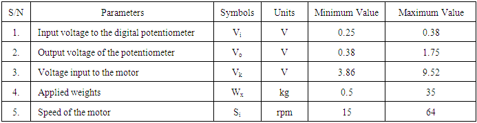
- The dynamic parameters of the electromechanical motor system are listed in Table 1 with their respective minimum and maximum values. The data for the following dynamic parameters have been collected for this work:1). The input voltage to the digital potentiometer; Vi;2). The output voltage of the potentiometer in response to changes in the input; Vj;3). The actual voltage input to the motor; Vk;4). The input standards weights, Wx; and5). The corresponding measured speed of the motor (in revolution per minute) in response to the changes in the inputs (voltage and applied weights). Si.
|
2.3. Description of the EMS Input-Output Data
- The picture of the completely designed and constructed EMS is shown in Fig. 2 [26]. Weights were combined to give a range from 0.5 kg to 35 kg limited by the diameter of the bowl on the iron plate. The input voltages and the corresponding speed of the EMS as measured by the counter circuit are summarized in Table 2. The input voltages were first fixed for no load condition and the speed in rpm was recorded. Then the experiment was repeated for each of the applied weights keeping the voltages fixed and the respective speed (in rpm) as displayed by the digital counter. The minimum recorded rpm with no load is 18 rpm while with 35 kg weight the digital counter recorded 15 rpm with the minimum input voltage of 3.86 V. The maximum speed recorded is 64 rpm which occur at the highest supplied voltage of 9.5 V under no load condition but 51 rpm with 35 kg weights applied [26].
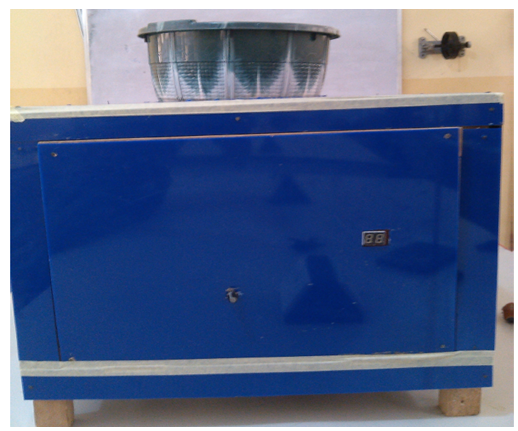 | Figure 2. The picture of the completely designed and constructed electromechanical motor system |
|
3. Formulation of the NN-Based MLMA and the Model Validation Algorithms for NNARMAX Model Identification
3.1. Formulation of the Neural Network Model Identification Problem
- The method of representing dynamical systems by vector difference or differential equations is well established in systems and control theories [3, 15, 27, 28]. Assuming that a p-input q-output discrete-time nonlinear multivariable system at time
 with disturbance
  can be represented by the following Nonlinear AutoRegressive Moving Average with eXogenous inputs (NARMAX) model:
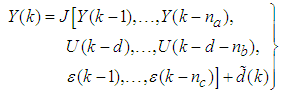 | (1) |
 is a nonlinear function of its arguments, and
  are the past output vector,
  are the past input vector,
  are the past noise vector,
  is the current output,
  are the number of past values of the system outputs, system inputs and noise inputs respectively that defines the order of the system, and
  is the time delay. The predictor form of (1) based on the information up to time
  can be expressed in the following compact form as [15]:
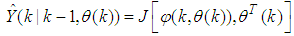 | (2) |

 is the regression (state) vector,
  is an unknown parameter vector which must be selected such that
  ,
,  is the error between (1) and (2) defined as
 | (3) |
 in
in  of (2) is henceforth omitted for notational convenience. Not that
  is the same order and dimension as
  .Now, let
  be a set of parameter vectors which contain a set of vectors such that:
 | (4) |
 is some subset of
  where the search for
  is carried out;
  is the dimension of
  ;
;  is the desired vector which minimizes the error in (3) and is contained in the set of vectors
  ;
;  are distinct values of
  ; and
; and  is the number of iterations required to determine the
  from the vectors in
  .Let a set of
  input-output data pair obtained from prior system operation over NT period of time be defined:
 | (5) |
 is the sampling time of the system outputs. Then, the minimization of (3) can be stated as follows:
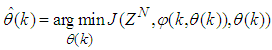 | (6) |
 is formulated as a total square error (TSE) type cost function which can be stated as:
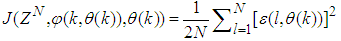 | (7) |
 as an argument in
  is to account for the desired model
  dependency on
  . Thus, given as initial random value of
  ,
,  ,
,  and (5), the system identification problem reduces to the minimization of (6) to obtain
  . For notational convenience,
  shall henceforth be used instead of
 .
.3.2. Neural Network Identification Scheme
- The minimization of (6) is approached here by considering
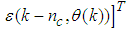
 as the desired model of network and having the DFNN architecture shown in Fig. 3. The proposed NN model identification scheme based on the teacher-forcing method is illustrated in Fig. 4. Note that the “Neural Network Model” shown in Fig. 4 is actually the DFNN shown in Fig. 3 via tapped delay lines (TDL). The inputs to NN of Fig. 4 are
 and
and 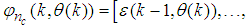
 which are concatenated into
 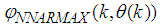 or simply
  as shown in Fig. 3. The output of the NN model of Fig. 4 in terms of the network parameters of Fig. 3 is given as:
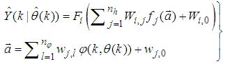 | (8) |
 and
and  are the number of hidden neurons and number of regressors respectively;
  is the number of outputs,
  and
and  are the hidden and output weights respectively;
  and
and  are the hidden and output biases;
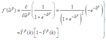
  is a linear activation function for the output layer and
  is an hyperbolic tangent activation function for the hidden layer defined here as:
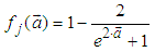 | (9) |
 is a collection of all network weights and biases in (8) in terms of the matrices
  and
and  . Equation (8) is here referred to as NN NARMAX (NNARMAX) model predictor for simplicity.
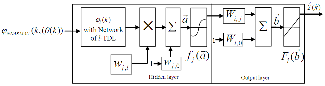 | Figure 3. Architecture of the dynamic feedforward NN (DFNN) model |
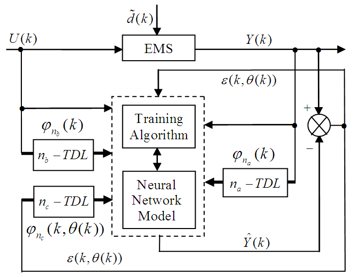 | Figure 4. NNARMAX model identification based on the teacher-forcing method |
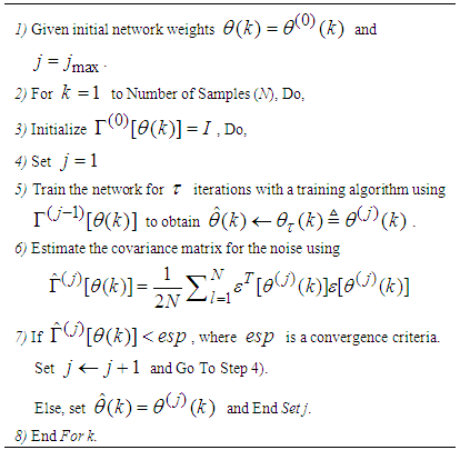
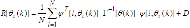
 in (1) is unknown but is estimated here as a covariance noise matrix,
 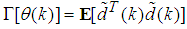 Using
Using , Equation (7) can be rewritten as [3], [15], [27]:
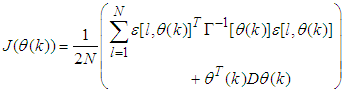 | (10) |
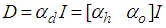 is a penalty norm and also removes ill-conditioning, where
  is an identity matrix,
  and
and  are the weight decay parameters for the input-to-hidden and hidden-to-output layers respectively. Note that both
  and
and  are adjusted simultaneously during network training with
  and are used to update
  iteratively. The algorithm for estimating the covariance noise matrix and updating
  is summarized in Table 3. Note that this algorithm is implemented at each sampling instant until
  has reduced significantly as in step 7).
|
3.3. Formulation of the NN-Based MLMA
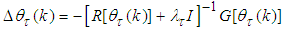
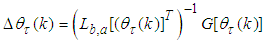
- Unlike the standard back-propagation (BP) algorithm which is a steepest descent algorithm, the MLMA algorithm proposed here is based on the Gauss-Newton method with the typical updating rule given from [3, 15, 27] as:
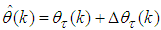 | (11) |
 | (12) |
 denotes the value of
  at the current iterate
 ,
,  is the search direction,
  and
and  are the Jacobian (or gradient matrix) and the Gauss-Newton Hessian matrices evaluated at
  .As mentioned earlier, due to the model
  dependency on the regression vector
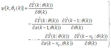
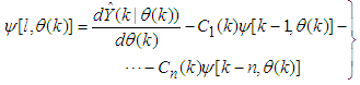
 , the NNARMAX model predictor depends on a posteriori error estimate using the feedback as shown in Fig. 4. Suppose that the derivative of the network outputs with respect to
  evaluated at
 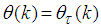 is given as [15]:
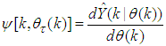 | (13) |
 | (14) |
 | (15) |
 , then (15) can be reduced to the following form [15]
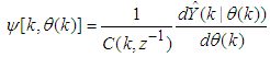 | (16) |
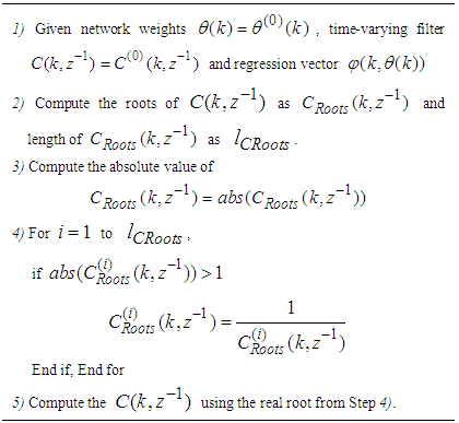
 which depends on the prediction errors based on the predicted outputs. Equation (16) is the only component that actually impedes the implementation of the NN training algorithms depending on its computation.Due to the feedback signals, the NNARMAX model predictor may be unstable if the system to be identified is not stable since the roots of (16) may, in general, not lie within the unit circle. The approach proposed here to iteratively ensure that the predictor becomes stable is summarized in the algorithm of Table 4. Thus, this algorithm ensures that roots of
  lies within the unit circle before the weights are updated by the training algorithm proposed in the next sub-section.
|
3.3.1. The Proposed Modified Levenberg-Marquardt Algorithm (MLMA)
- The Levenberg-Marquardt [28-30] modification to (12) is the inclusion of a non-negative parameter
 to the diagonal of
  with a new iterative updating rule as follows:
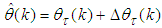 | (17) |
 | (18) |
 and
and  are:
are: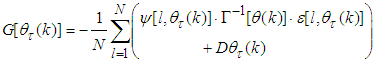 | (19) |
 | (20) |
 the derivative of the network outputs with respect to
  evaluated at
  and is computed according to (16).The parameter
  characterizes a hybrid of searching directions and has several effects [7, 29-32]: 1) for large values of
  (18) becomes steepest descent algorithm (with step
  ) which requires a descend search method; and 2) for small values of
  (18) reduces to the Gauss-Newton method and
 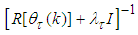 may become non-positive definite matrix.Despite the fact that (10) is a weighted criterion, the convergence of the Levenberg-Marquardt algorithm (LMA) may be slow since
  contains many parameters of different magnitudes, especially if these magnitudes are large as in most cases [8, 10, 28]. This is the major reason for not using the LMA in online training of the NNs.This problem can be alleviated by adding a scaling matrix
  (where
  is the scaling parameter and
  is an identity matrix) which is adjusted simultaneously with
 and instead of checking
 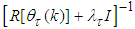 in (18) for positive definiteness, the check is expressed as
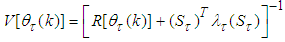 | (21) |
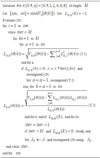
 is chosen. Different from other methods [28, 32-34] the method proposed here uses the Cholesky factorization algorithm and then iteratively selects
  to guarantee positive definiteness of (21) for online application. First, (21) is computed and the check is performed. If (21) is positive definite, the algorithm is terminated, otherwise
  is increased iteratively until this is achieved. The method is summarized in Table 5. The key parameter in the algorithm is
 . Next, the Cholesky factor
  given by (T.2) in Table 5 is reused to compute the search direction from (18) in two-stage forward and backward substitution given respectively as:
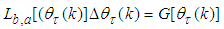 | (22) |
 | (23) |
|

 is too far from the optimum value
 . Thus, the LMA is sometimes combined with the trust region method [35] so that the search for
  is constrained around a trusted region
 . The problem can be defined as [3, 15]:
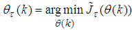 | (24) |
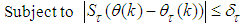 | (25) |
 is the second-order Gauss-Newton approximate of (10) which can be expressed as:
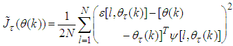 | (26) |
 . Thus, with this combined method and using the result from (23), Equation (17) can be rewritten as
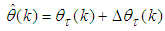 | (27) |
 and
and  has led to the coding of several algorithms [7, 28-34]. In stead of adjusting
  directly, this paper develops on the indirect approach proposed in [35] but reuses
  computed in Table 5 to update the weighted criterion (10). Here,
  is adjusted according to the ratio
  between the actual reduction of (10) and theoretical predicted decrease of (10) using (26). The ratio can be defined as:
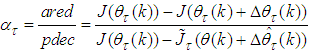 | (28) |
 in (10) for convenience and
 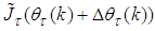 is the Gauss-Newton estimate of (10) using (26).The complete modified Levenberg-Marquardt algorithm (MLMA) for updating
  is summarized in Table 6. Note that after
  is obtained using the algorithm of Table 6, the algorithm of Table 3 is implemented until the conditions set out in Step 7) of the algorithm are satisfied.
|

3.4. Proposed Validation Methods for the Trained NNARMAX Model
- Network validations are performed to assess to what extend the trained network has approximated and capture the operation of the underlying dynamics of a system and as measure of how well the model being investigated will perform when deployed for the actual process [3, 15, 27].The first test involves the comparison of the predicted outputs with the true training data and the evaluation of their corresponding errors using (3).The second validation test is the Akaike’s final prediction error (AFPE) estimate [3, 15, 17, 28, 34] based on the weight decay parameter D in (10). A smaller value of the AFPE estimate indicates that the identified model approximately captures all the dynamics of the underlying system and can be presented with new data from the real process. Evaluating the
 portion of (3) using the trained network with
  and taking the expectation
  with respect to
  and
and  leads to the following AFPE estimate [3], [15], [27]:
 | (29) |
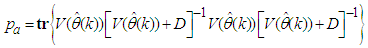 and
and  is the trace of its arguments and it is computed as the sum of the diagonal elements of its arguments,
 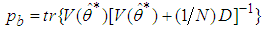 and
and  is a positive quantity that improves the accuracy of the estimate and can be computed according to the following expression:
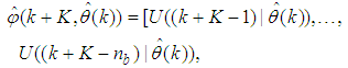
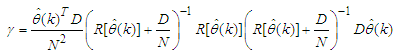 The third method is the K-step ahead predictions [10] where the outputs of the trained network are compared to the unscaled output training data. The K-step ahead predictor follows directly from (8) and for
 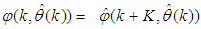 and
and  , takes the following form:
 | (30) |

 The mean value of the K-step ahead prediction error (MVPE) between the predicted output and the actual training data set is computed as follows:
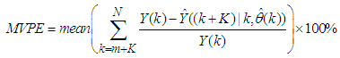 | (31) |
 corresponds to the unscaled output training data and
  the K-step ahead predictor output.
4. Dynamic Modeling and Adaptive Closed-Loop Simulations of the EMS Using Discrete-Time PID Controller
4.1. Selection of the Manipulated Inputs and Controlled Outputs for the Dynamic EMS Modeling Problem
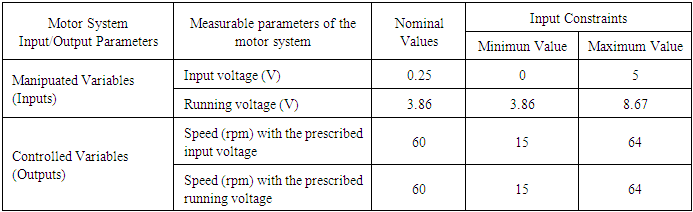
- The manipulated variable (MV) is the variable chosen to affect control over an output variable. As the output is being controlled it is normally referred to as the controlled variable (CV). The objective of a control system is to keep the CV at their desired values (or setpoints). This is achieved by manipulating the MV using a control algorithm [36]. The manipulated variables with the nominal values and constraints as well as the controlled variable with the nominal values and the constraints are as shown in Table 2. The manipulated variable is the input voltage to the digital potentiometer and the running voltage of the motor with nominal values of 0.25 V and 3.86 V respectively (see Tables 1 and 2). The controlled variable is the desired output rpm of the motor with nominal value of 60 rpm.Disturbances are variables that fluctuate and cause the process output to move from the desired operating value (setpoint). A disturbance could be a change in flow or temperature of the surroundings or pressure etc. Disturbance variables can normally be further classified in terms of measured or unmeasured signals. The different random weights applied to the EMS serves as the disturbance introduced to the system for the study and it ranges from 0.5 kg to 35 kg. More weights could be accommodated for further studies but the diameter of the bowl would need to be increased and the complete design of the EMS would require total adjustments.
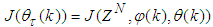
4.2. Formulation of the EMS NNARMAX Model Identification and Prediction Problem
4.2.1. Statement of the EMS Neural Network-Based Model Identification Problem
- The development of accurate system models from first-principles or analytically for dynamical systems could be difficult and/or frustrating if not practically impossible [3, 15]. The modeling task becomes even more challenging for systems with relatively short sampling time such as the EMS considered in this study with an approximate sampling time of 16 milliseconds. However, the emergence of NNs simplified the process of capturing relatively accurate dynamic discrete-time models of dynamical systems based on the availability of either only input, only output or input-output data [1-15]. This sub-section develops on Sections 2 and 3.Thus, from the discussions so far, the only measured input that influence the behaviour of the EMS is the input voltage (Vi) given by:
 | (32) |
 | (33) |
 for the NNARMAX model predictor discussed in Section 3 and defined here as follows:
 | (34) |
 | (35) |
 | (36) |
 | (37) |
 | (38) |
4.2.2. Experiment with EMS for Neural Network Training Data Acquisition
- Based on previous discussions, the PMDC–based EMS can be considered as a SISO system, thereby eliminating the complications associated with a MIMO systems [41]. The input to the electromechanical system is an electrical voltage sent to the PMDC motor while the output is the rpm of the PMDC motor measured by an opto-sensor. The input-output measurements (data) obtained from the electromechanical system was used for the development of dynamic models which was used for the adaptive controllers design, since the dynamic model of the system will ensure stability in situations where the system operates outside the normal operating conditions. For the purpose of neural network modeling of the system, a total of 476 data samples were obtained from the experiments performed on the designed and constructed EMS developed in [26]. Of the 476 experimental data acquired from the EMS, 381 data (representing 80%) is for the NN training while the remaining 95 data (representing 20%) have been reserved for the trained NN model validation. The entire simulation of the EMS is achieved using MATLAB and Simulink® software from The MathWorks [42].
4.2.3. Formulation of the Error Back-Propagation with Momentum (EBPM) Algorithm
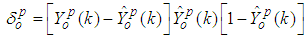
- In order to investigate the performance of the proposed MLMA, the so-called error back-propagation with momentum (EBPM) algorithm is used for this purpose. The EBPM algorithm is a variation of the standard back-propagation algorithm originally proposed by [37] which has been modified in [15] for use in this paper. The EBPM algorithm is summarized from [15] as follows:1). The weight of a connection is adjusted by an amount proportional to the product of an error signal
 , on the unit k receiving the input and the output of the unit
  sending the signal along the connection as follows:
 | (39) |
 | (40) |
 defined in (9), the output
  can be expressed as:
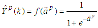 | (41) |
 | (42) |
 | (43) |
 | (44) |
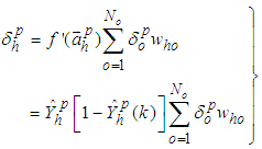
 expressed as:
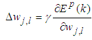 | (45) |
 in (39) and (45) is chosen as large as possible without leading to oscillation. To avoid oscillation at large
  , the change in weight is made to be dependent on past weight change by adding a momentum term as follows:
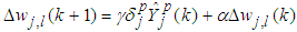 | (46) |
 indexes the presentation number and
  is a constant which determines the effects of the previous weight change. When no momentum term is used, it can take a long time before the minimum is reached with a low learning rate, whereas for high learning rates the minimum is never reached because of the oscillations. When a momentum term is added, the minimum is reached faster [38-40].
4.2.4. Scaling the Training Data and Rescaling the Trained Network that Models the EMS
- Due to the fact the input and outputs of a process may, in general, have different physical units and magnitudes; the scaling of all signals to the same variance is necessary to prevent signals of largest magnitudes from dominating the identified model. Moreover, scaling improves the numerical robustness of the training algorithm, leads to faster convergence and gives better models. The training data are scaled to unit variance using their mean values and standard deviations according to the following equations [3, 15, 27]:
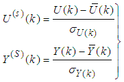 | (47) |

 and
and  ,
,  are the mean and standard deviation of the input and output training data pair; and
  and
and  are the scaled inputs and outputs respectively. Also, after the network training, the joint weights are rescaled according to the expression
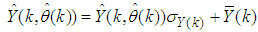 | (48) |
 and
and  shall be used in the discussion of results.
4.2.5. Training the Neural Network that Models the EMS
- The NN input vector to the neural network (NN) is the NNARMAX model regression vector
 defined by (37). The input
  , that is the initial error estimates
  given by (3), is not known in advance and it is initialized to small positive random matrix of dimension
  by
by  . The outputs of the NN are the predicted values of
  given by (8).For assessing the convergence performance, the network was trained for
  = 20 epochs (number of iterations) with the following selected parameters:
  ,
,  ,
,  ,
,  ,
,  ,
,  (NNARMAX),
  ,
,  ,
,  and
and  . The details of these parameters are discussed in Section 3; where
  and
and  are the number of inputs and outputs of the system,
  and
and  are the orders of the regressors in terms of the past values,
  is the total number of regressors (that is, the total number of inputs to the neural network),
  and
and  are the number of hidden and output layers neurons, and
  and
and  are the hidden and output layers weight decay terms. The two design parameters
  and
and  were selected to initialize the MLMA algorithm. The maximum number of times the algorithm of Table 3 is implemented is 6 in all the simulations; that is
 . For the EBPM, the two design parameters are selected as
  and
and  .The 381 training data is first scaled using equation (47) and the network is trained for τ = 20 epochs using the proposed MLMA and the EBPM algorithm proposed in Sections 3.3 and 4.2.3 respectively.
4.3. Validation of the Trained NNARMAX Model for the Modeling and Prediction of the EMS Dynamics
- According to the discussion on network validation in Section 3.4, a trained network can be used to model a process once it is validated and accepted, that is, the network demonstrates its ability to predict correctly both the data that were used for its training and other data that were not used during training. The networks trained with the EBPM and the proposed MLMA algorithms needs to be validated with proposed three different methods by the use of scaled and unscaled 381 training data as well as with the 95 data reserved for the validation of the trained network for the EMS.The three different validation techniques used to evaluate the performances of the two trained networks are: 1). one-step ahead prediction of the scaled training data; 2). one-step ahead prediction of the unscaled validation data; 3). K-step ahead prediction of the unscaled training data; and 4). Akaike’s final prediction error (AFPE) estimate.
4.3.1. Network Training of the EMS Using EBPM and the Proposed MLMA Algorithms
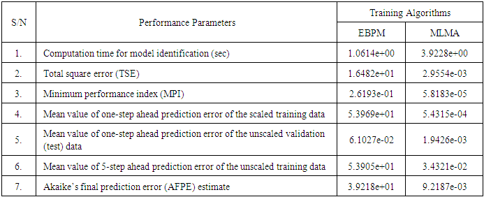
- The two training algorithms used here are the EBPM and the proposed MLMA algorithms discussed in Sections 4.2.3 and 3.3 respectively. The training data is first scaled according to equation (47) and the network is trained using the two algorithms.After network training, the trained network is again rescaled according to (48) so that the resulting network can work with unscaled EMS real-time data. The performances of the EBPM and the MLMA algorithms are shown in Fig. 5 through Fig. 7 while the Table 7 presents the summary of the training and validation results for quick comparison.The computation time for training the networks using each of the algorithms are shown in the first row of Table 7.
|
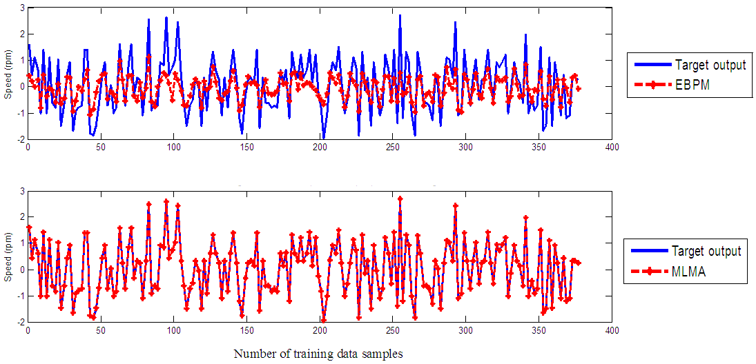 | Figure 5. One-step ahead output prediction of scaled training data |
4.3.2. One-Step Ahead Predictions Simulation for the EMS
- In the one-step ahead prediction method given by (8), the scaled training data are compared with the one-step ahead output predictions of the trained network and an assessment of their corresponding errors is made. The comparison of the one-step ahead predictions of the scaled training data (target output, blue ––) against the trained network output predictions (red --*) by the networks trained for 20 epochs using the EBPM and the MLMA algorithms are shown in Fig. 5.The mean value of the one-step ahead prediction errors for the prediction of the scaled training data by the network trained using the EBPM and the MLMA algorithms are given in the fourth row of Table 7. It can be seen in Fig. 5, the network predictions of the training data based on the network trained using the MLMA algorithm closely match the original training data used whereas there are much prediction mismatch obtained with the network trained using the EBPM algorithm. Also, the smaller one-step ahead prediction error obtained using the network trained by the MLMA when compared to that by EBPM algorithm are also evident in the fourth row of Table 7. This error is an indication that the trained networks using the MLMA algorithm captures and approximates the nonlinear dynamics of the EMS accurately. This is further justified by the small mean value of the TSE obtained using MLMA algorithms given in the second row of Table 7.Furthermore, the suitability of the EBPM and proposed MLMA algorithms for NN model identification for use in the EMS is investigated by validating the trained network with 95 unscaled test data. The comparison of the trained network predictions (red --*) of the test data with the actual test data (test data, blue ––) for 20 epoch are shown in Fig. 6 for the EBPM and the MLMA algorithms. It is evident that the unscaled test data predictions by network trained using the MLMA algorithm match the true test data to a high accuracy when compared to that obtained by the network trained using EBPM. The superior performance of the proposed MLMA algorithm over the EBPM algorithm proves the effectiveness of the proposed MLMA approach.The one-step ahead prediction accuracies of the unscaled test data by the networks trained using the EBPM and the MLMA algorithms is evaluated by the computed mean prediction errors shown in the fifth row of Table 7. It can be seen that the one-step ahead test data prediction errors by the network trained using MLMA algorithm are much smaller than those obtained from the network trained using the EBPM algorithm.This one-step ahead unscaled validation data prediction results given by Fig. 6 as well as the mean value of the one-step ahead prediction error of the validation data shown in the fifth row of Table 7 justify that the network trained using the MLMA algorithm mimic the dynamics of the electromechanical system and that the resulting network can be used to model the actual EMS in an industrial environments and/or in real life scenarios.
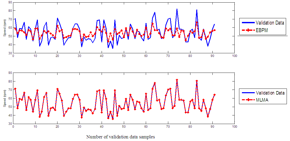 | Figure 6. One-step ahead output prediction of unscaled validation (test) data |
4.3.3. K–Step Ahead Prediction Simulations for the EMS
- The results of the K-step ahead output predictions (red --*) using the K-step ahead prediction validation method for 5-step ahead output predictions (K = 5) compared with the unscaled training data (target output) are shown in Fig. 7 for the network trained using the EBPM and MLMA algorithms. The value K = 5 is chosen since it is a typical value used in most model predictive control (MPC) applications. The comparison of the 5-step ahead output predictions performance by the network trained using EBPM and the MLMA algorithms shows the superior performance of the MLMA algorithm over the EBPM algorithms for use in distant or multi-step ahead predictions. The computation of the mean value of the K-step ahead prediction error (MVPE) using equation (31) gives 5.3905×10+01 and 3.4321×10-02 respectively by the network trained using the EBPM and MLMA algorithms as shown in the sixth row of Table 7. The relatively smaller MVPE obtained by the network trained with the MLMA algorithm is indications that the trained network approximates the dynamics of the EMS to a high degree of accuracy.
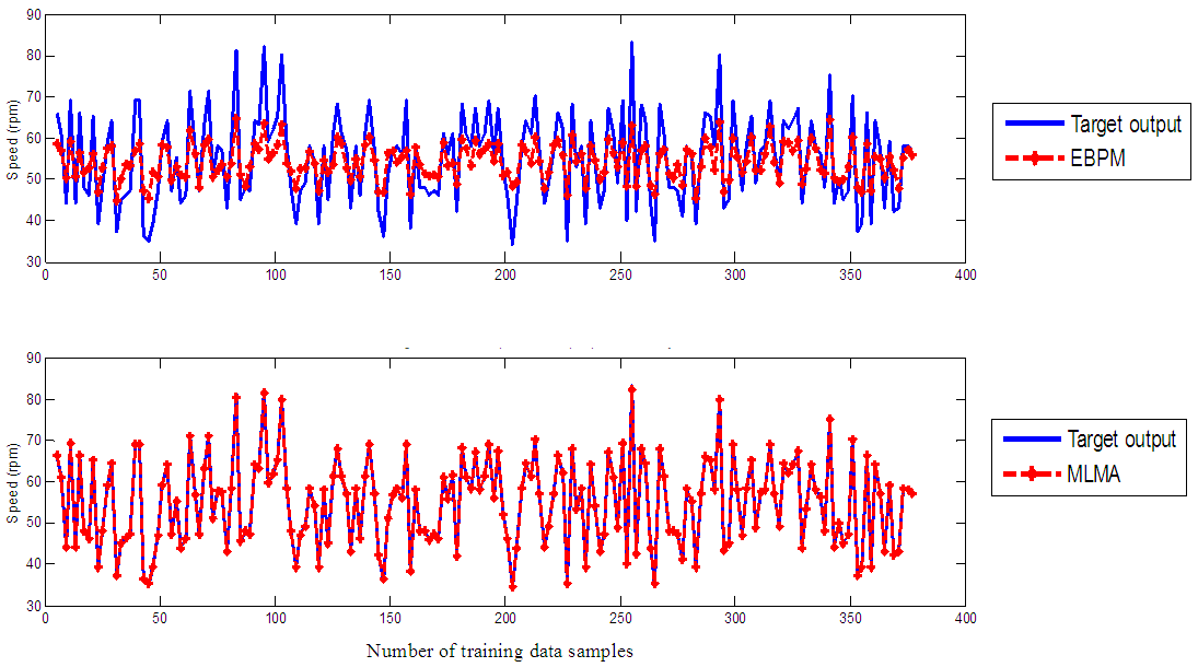 | Figure 7. Five-step ahead output prediction of unscaled training data |
4.3.4. Akaike’s Final Prediction Error (AFPE) Estimates for the EMS
- The implementation of AFPE algorithm discussed in chapter four and defined by equation (29) for the regularized criterion for the network trained with the EBPM and the MLMA algorithms with multiple weight decay gives the respective AFPE estimates of the two algorithms as shown in the seventh row of Table 7.These small values of the AFPE estimate indicate that the trained networks capture the underlying dynamics of the EMS and that the network is not over-trained [3, 15, 27]. This implies that optimal network parameters have been selected including the weight decay parameters. Again, the results of the AFPE estimates obtained with the networks trained using the MLMA algorithm are by far smaller when compared to that obtained using EBPM algorithm.
4.4. Dynamic Model Validation and Closed-Loop Simulations of the EMS Using PID Controller
- Besides the training of the NN model with static data taken from plant tests, it would be of interest to validate the prediction accuracy of a trained network under the same dynamic conditions in which the system is operating in the presence of a disturbance
 .Disturbances are variables that fluctuate and cause the process outputs to move from the desired operating values (set-points or desired trajectories). The prescribed desired speed trajectory specified for the EMS is 60 rpm which must be maintained irrespective of the applied weight(s). A disturbance could be a change in flow or temperature of the surroundings or pressure etc. Disturbance variables can normally be further classified in terms of measured or unmeasured signals. The different weights (in kg) applied in this research serves as the disturbances introduced randomly to the EMS and it ranges from 0.5 kg to 35 kg.
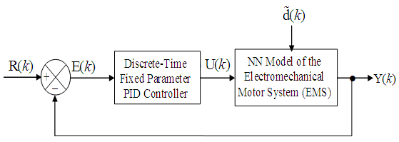 | Figure 8. The Discrete-time PID control scheme |
 is:
is: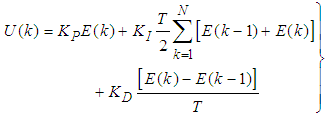 | (49) |
 and
and  are the proportional, integral and derivative gains respectively,
  is the sampling time and
 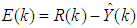 is the error between the desired reference
  and predicted output
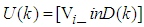
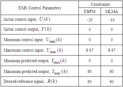
 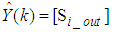 and N is the number of samples. The minimum and maximum constraints imposed on the PID controller to penalize changes on the EMS control inputs
  and outputs
  are given as:
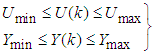 | (50) |
 ,
,  and
and  for Si_out ( in rpm). The constraints imposed on the EMS defined in (50) are summarized in Table 8 together with the initial control inputs and outputs.
|
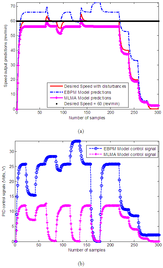 | Figure 9. Closed-loop PID control performance of the EMS using NN model trained with EBPM and MLMA algorithms: (a) output speed predictions and (b) control signals |
5. Conclusions and Future Directions
- This paper presents a novel technique for the dynamic modeling of an electromechanical motor system (EMS) and the closed-loop prediction of EMS behaviour in the presence of disturbances using an advanced online nonlinear model identification algorithm called the modified Levenberg-Marquardt algorithm (MLMA) based on artificial neural networks for the nonlinear model identification of an EMS. The paper also presents the complete formulation of the proposed MLMA.In order to investigate the performance of the proposed MLMA algorithm, the error back-propagation with momentum (EBPM) algorithm is implemented and its performance compared with proposed MLMA. The simulation results from the application of these algorithms to the dynamic modeling of the EMS as well as the validation results show that the neural network-based MLMA outperforms the EBPM algorithm with much smaller predictions error and good tracking abilities with high degree of accuracy.The simulation results from the dynamic modeling in closed-loop with a discrete-time fixed parameter PID control shows that the proposed MLMA model identification algorithm can be used for the EMS in real life scenarios and/or in industrial environments.Although, it is evident the performance of the PID controller is not satisfactory due to poor tracking of the desired trajectory with to oscillations below the desired trajectory. Thus, the next aspect of the work could be on the development of efficient adaptive control algorithms to replace the fixed-parameter PID controller for the EMS so as to obtain an adaptive electromechanical speed control system.