1. Introduction

The dynamic behavior of the direct current (d.c.) motor is mainly determined by the type of the connection between the excitation winding, the armature winding including the commutation and compensation windings. It has been shown that d.c. motors are most suitable for wide range speed control and are therefore used in many adjustable speed drives [1-6]. They also explained that a linear model of a simple d.c. motor consists of an electrical equation and mechanical equation using Kirchhoff’s voltage law (KVL) and Newton’s second law while the speed can be controlled by controlling the armature voltage, armature resistance and the flux. The speed control using armature resistance by adding external resistor is not used very widely because of the large energy losses due to the resistance. The armature voltage control is normally used for speeds of up to rated speed (base speed) while Flux control is used for speed beyond rated speed but at the same time the maximum torque capability of the motor is reduced since for a given maximum armature current, the flux is less than the rated value and as such the maximum torque produced is less than the maximum rated torque.

The dynamic and steady-state model of separately excited d.c. motor is needed to analyse the torque speed characteristics. The set of equations presented in [3-7], constitutes a model of the d.c. motor, which may be represented as a nonlinear dynamic system. The main restrictions of this model, with respect to a real motor are the assumption that the magnetic circuit is linear (such an assumption is approximate). While in a d.c. motor, the magnetic flux is generated by windings located on the stator, the magnetic field arises from the stator coils which rotate with respect to the stator by increasing the number of coils and by a more sophisticated supply.

Also, the motor exerts a torque, while supplied by voltages on the stator and on the rotor. This torque acts on the mechanical structure, which is characterized by the rotor inertia and the viscous friction coefficient; gears are introduced between the motor and the load, thus reducing by a factor in the angular velocity of the load itself when the speed required by the load is too low as compared to the nominal speed of the motor [3-6, 8].

Direct current motors are usually modeled as linear systems and then linear control approaches are implemented [9-12]. However, most linear controllers have unsatisfactory performance due to the changes of motor-load dynamics and due to nonlinearities introduced by the armature reaction. Neglecting the impact of external disturbances and of nonlinearities may risk the stability of the closed loop system. For this reason, the d.c. motor control using the conventional proportional-integral-derivative (PID) controllers are inadequate and more effective control approaches are needed [13-15].

Traditionally, the d.c. motors and the associate close loop control systems used to drive them have been emboweled using classic control theory techniques, based on transfer functions. Control system design and analysis technologies are widely suppressed and very useful to be applied in real-time development. Some can be solved easily by hardware technology and by the use of advanced software control systems with detailed analysis and specifications [16].

Modelling of any kind of system can be based on one of following two main principles: 1). Modelling from fundamental physical principles (analytical modelling) if the physical laws describing the system behaviour is known and equations can be derived. Both linear and nonlinear phenomena can be modelled including e.g. non-smooth dynamics. Usually, the remaining problems are: a) parameter estimation of proposed model; b) validation of the model. A good example of such system is the pendulum, where the equation is easy to derive, but e.g. the viscous damping parameter could be difficult to guess. Moreover, when the model is validated using experimental data measured on real pendulum, the dry friction can appear significant and model must be reformulated. 2). Modelling from measured data with random coloured noise (stochastic modelling). If the system physics is unknown or difficult to express, the model can be derived from experimental data measured on real system. The linear discrete time model with particular noise model is usually assumed and the identification algorithm searches for its coefficients. Also other techniques such as artificial neural networks can be used as general approximator for the system modelling. The description of dry friction or other non-smooth behaviour is problematic.

The second approach is supposed to be more adequate for the electromechanical system modelling. The electromechanical system can usually be considered as system with lumped parameters for which mechanical and electrical equations are simple and easy to derive. Many of such parameters are usually measured directly or indirectly [17, 18].

In order to develop an efficient adaptive control scheme for the adaptive speed control of the electromechanical motor system, the complete design and construction of the electromechanical motor system is first necessary. Section 2 presents the material and detailed methodology employed in the design and construction of the electromechanical motor system. The calibration and experimental data collection from the designed and constructed electromechanical motor system are presented in Section 3. Section 4 concludes the paper with some major highlights on the contributions of the proposed design techniques as well as insights on future directions.

2. Materials and Methodology

This section presents the development and the design of the proposed electromechanical system with details of the materials used for the construction. Section 2.2 presents the circuit description of the designed power supply, driver circuit, signal amplifier circuit as well as the electronic digital circuit used in this work. In section 3 the experimental details on the data collection from the electromechanical system is presented. The measurement procedure with the description of the electromechanical input-output data that describes the system behaviour, the considerations of the electromechanical system and the effects of the process variables on the system are also presented in the same Section 3.

2.1. Design of the Electromechanical Motor System

The actuator used in this project is a PORCHE PPWPM432 windshield wiper motor which has a worm gear and simple ring gear that gives the device its incredible torque. This type of motor is called a “gearhead” or "gear motor" and has the advantage of having lots of torque. The system has been designed to accommodate different standard weights which are to be loaded through the bowl fitted to the iron sheet plate with bolts and nuts to hold it firmly as it rotates. The sheet (46 cm diameter, 0.1 cm thickness) is welded to the motor system with a shaft connected to the motor through the gearing system which transfers the motion of the motor to the bowl. Bearings were fitted to allow for free movements or rotation of the system and balancing rods were clamped to hold the system from falling and to maintain balance while rotating. The light dependent resistor (LDR) sensor is installed and aligned with the light source to receive the incident light through the hole of 2.5 cm bored on the sheet. The following is a list and specification of materials used for the design of the proposed electromechanical motor system, namely: 1). a PORCHE PPWPM432 windshield wiper motor with 19.6 cm diameter; 2). a container bowl with 21 cm height, 18.8 cm bottom diameter and 30 cm top diameter; 3). an iron sheet plate of 46 cm diameter, 0.1 cm thickness with a 2.5 cm hole for the sensor; 4). two gears 45 teeth and 35 teeth with 4.5 cm diameter and 3.5 cm diameter respectively; and 5). an Iron shaft of 19.4 cm length and 5.1 cm diameter.

The sensor and bulb are installed at the bottom and top respectively with 4.5 cm equidistant from the iron sheet plate. A well labelled schematic diagram of the proposed electromechanical motor system is shown in Fig. 1(a) and a well labelled 3-D diagram of the proposed electromechanical motor system is also shown in Fig. 1(b) for a 3D view of the system.

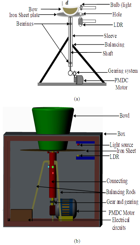Figure 1. The designed electromechanical motor system: (a) Schematic drawing of the electromechanical system and (b) 3-D drawing of the electromechanical speed control system

2.2. Description of the Electronic Circuit

The standard voltage rating for the PMDC motor is 12 V direct current (d.c.). The electrical system in a running automobile usually puts out between 13 and 13.5 V, so it is safe to say the motor can safely handle up to 13.5 V with and the minimum required current is about 1.6 A for the motor spinning with no load. As other mechanical loads are added, the current it is expected to increase dramatically, doubling or even tripling under a heavy load. (when testing for torque, it was discovered that the motor could draw close to 14 A in a stalled condition). This factor was taken into account when designing the power supply. Since the motor uses only what it needs when it comes to current, it is best to provide a source with a higher current rating than it might need from a minimum of 5 A or more to handle most circumstances. When power is applied, the motor runs in a jerky motion because the motor draws more current in the few moments when it first starts up (called inrush current). With some low current switching power supplies, this may trigger the circuitry which is designed to protect the supply. The power supply senses an over-current condition and shuts down. It then restarts, once again senses over-current and shuts down. This pattern continues repeatedly which causes the jerky motor operation. The motor could damage the power supplies due to back electromotive force (e.m.f.) when switched off, so it requires a clamp diode connected across the motor in the reverse direction. The running current of the motor was measured using a 12 V car battery and an ammeter. A digital multimeter set at the 10 amps d.c. range was used to measure the current. The complete circuit diagram for the system is presented in Fig. 3.

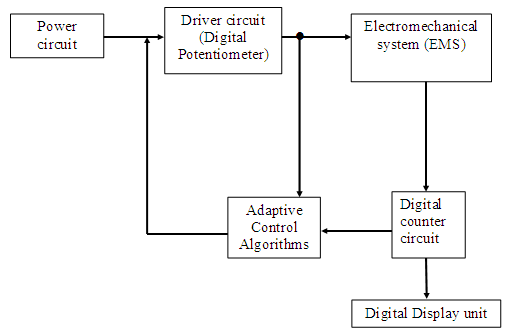Figure 2. Block diagram of the proposed electromechanical motor speed control system

2.2.1. The 12-V Regulated Power Supply Unit

The circuit of Fig. 3 is to be powered by a high current 12 V power supply as the motor draws high current especially at start up. The Power supply uses LM7812 integrated circuit (IC) as the voltage regulator IC (U1) and can deliver up to 25 A to the load by the help of the cascaded five TIP2955 pass transistors (Q1 to Q5). Each transistor can handle up to 5 A and five of them result a total output current of 25 A. In this design the regulator IC delivers about 800 mA. A diode (D1) is connected after the LM7812 to protect the IC against high current transients. The transistors and the 12 V regulator IC both are adequately mounted on a heat sink. Also, when the load current is high, the power dissipation of each transistor increases and excess heat may cause the transistors to fail; thus the need for the heat sink to serve as a cooling device for the transistors. The 100 Ω (R6) and 0.47 Ω 5 Watts limiting resistors (R1 to R5 choke resistors) are used for stability and prevent current swamping as the tolerances of d.c. current gain will be different for each transistor. The bridge rectifier IC (BR1) is capable of passing up to 100 A.

The input transformer (TR1) is a 220 V to 18 V step down transformer rated 12 V and can deliver very high current. The next stage uses the 60 A, 1000 V bridge rectifier cross to rectify the a.c. to d.c. and a large capacitor (C1) 4700 µF rated 50 V to filter the d.c. signals output from the rectifier circuit from ripples. The input voltage to the regulator is about 18 V so it is a bit higher than the output voltage (12 V) so that the regulator can maintain its output. The LM7812 IC will only pass 1 amp or less of the output current, the remainder being supplied by the outboard pass transistors. As the circuit is designed to handle loads of up to 25 A, then the five TIP2955 are wired in parallel to meet this demand. The dissipation in each power transistor is one fifth of the total load, but adequate heat sinking is mounted. In the event that the power transistors should fail, then the regulator would have to supply full load current and would fail with catastrophic results. A diode in the regulator output provides a safeguard for the components of the power supply especially the regulator and the power transistors against back e.m.f. from the motor [19].

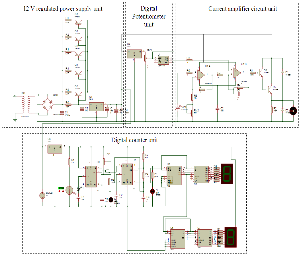Figure 3. The complete circuit diagram of the electronic part of the system

2.2.2. The Digital Potentiometer Unit

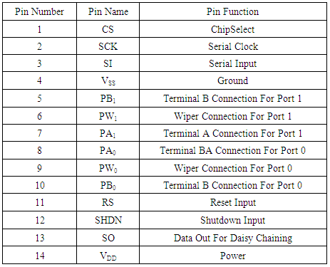
The key to this circuit unit is a low-power digital potentiometer IC (U2), 100 kΩ version (MCP42100). A digital Potentiometer is a digitally controlled device that can be used to adjust voltage or current and offers the same analog functions as a mechanical potentiometer or rheostat. This allows an automatic calibration process that is more accurate, robust, and faster, with smaller voltage glitches. Digital Potentiometers are often used for digital trimming and calibration of analog signals and are typically controlled by digital protocols, such as I2C and SPI, as well as more basic up/down and push-button protocols [20].

Architecture of the MCP42100 Digital Potentiometer

A digital Potentiometer is a 3-terminal device with an internal architecture that is comprised of an array of resistances and switches. Each digital Potentiometer consists of passive resistors in series between terminals A and B as shown in Fig. 4 (a). The wiper terminal, W, is digitally programmable to access any one of the 2n-tap points on the resistor string. The resistance between terminals A and B, R_AB, is commonly called the end-to-end resistance. ADI offers a wide range of end-to-end resistor options spanning from 1 kΩ to 1 MΩ.

The resistance between terminals A and W, R_AW, and the resistance between terminals B and W, R_WB, are complementary. That is, if R_AW increases, then R_WB will decrease in the same proportion. There is no restriction on the voltage polarity applied to terminals A, B, or W. Voltage across the terminals A to B, W to A, and W to B can be at either polarity–the only requirement is to ensure that the signal does not exceed the power supply rails. Similarly, there is no limitation in the current flow direction; the only restriction is that the maximum current does not exceed the current density specification, typically on the order of a few mA.

The MCP42100 has 256- position and contains two independent channels in a 14-pin PDIP, SOIC or TSSOP package Fig. 4(b). The wiper position varies linearly and is controlled via an industry-standard SPI interface. The devices consume less than 1 μA during static operation. A software shutdown feature is provided that disconnects the “A” terminal from the resistor stack and simultaneously connects the wiper to the “B” terminal. In addition, it has a SHDN pin (see Fig. 4(b) and Table 1) that performs the same function in hardware. During shutdown mode, the contents of the wiper register can be changed and the potentiometer returns from shutdown to the new value. The wiper is reset to the mid-scale position upon power-up. The RS (reset) pin implements a hardware reset and also returns the wiper to mid-scale. The MCP42100 SPI interface includes both the SI and SO pins, allowing daisy-chaining of multiple devices. Channel- to-channel resistance matching on the MCP42100 varies by less than 1%. These devices operate from a single 2.7 – 5.5 V supply and are specified over the extended and industrial temperature ranges.

In the potentiometer mode Fig. 4(a), all three terminals of the device are tied to different nodes in the circuit. This allows the potentiometer to output a voltage proportional to the input voltage. Configured in the potentiometer mode Fig. 4(b), this IC provides an output discrete voltage steps between its minimum and maximum settings (0 V and 5 V). A low-power linear regulator (LM7805) provides a +5 V supply rail for MCP42100 (whose maximum rating is +5 V).

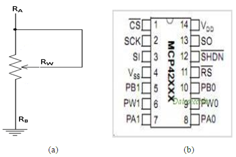Figure 4. (a) Potentiometer mode of the MCP42100 and (b) pin description of the MCP42100

Table 1. The MCP42100 digital potentiometer pin description

The output voltage and current of from the wiper of the digital potentiometer is observed to span between 0 V and 2 V and thus was not enough to turn on the base of the transistor (Q6) 2N3053 and so there is need for a suitable amplifier. In this design project, an OP284 rail-to-rail operational amplifier (U4:A&B) at the output of the digital potentiometers was used for the amplification. Potentiometers are often used to adjust system reference levels or gain. Programmable gain circuits using digital potentiometers can be realized in a number of different ways. Due to the high input impedance of the amplifier, the wiper resistance is not included in the transfer function.

Digital Potentiometer Output Voltage Amplification

The output voltage and current of from the wiper of the digital potentiometer is observed to span between 0 V and 2 V and thus is not enough to turn on the base of the transistor (Q6) 2N3053 and so there is need for a suitable amplifier.

To provide 0 V to +12 V outputs as required by the motor controller, a single-supply, rail-to-rail operational amplifier (op-amp) OP284 (U4) amplifies the MCP42100 output by a factor of two. The input common-mode range for this op amp, (250 mV beyond either supply rail), allows it to generate 0 V to +10 V outputs like a mechanical potentiometer. The resistors R14 and R13 set the op-amp gain to 2 V/V (see Fig. 3). The circuit's low quiescent current ranges from 86 µA for a 0 V output to 186 µA at +10 V.

In this design, a rail-to-rail operational amplifier (OP284) is used for amplification at the output of the digital potentiometers. The OP284 is a low noise dual op amp with a bandwidth of 4 MHz and rail-to-rail input/output operation [21]. These properties make it ideal for low supply voltage applications such as in a two op amp instrumentation amplifier as shown in Fig. 5. The circuit uses the classic two op-amp instrumentation topology with four resistors to set the gain as in Fig. 5(a) while the pin description is shown in Fig. 5(b). The transfer equation of the circuit is identical to that of a non-inverting amplifier. Resistors R13 and R9 should be closely matched to each other as well as to resistors (R14 and RV2) and R10 to ensure good common-mode rejection (CMR) performance. It is advisable to use resistor networks for R8 and R9, because these exhibit the necessary relative tolerance matching for good performance. Potentiometer RV2 is used for optimum d.c. CMR adjustment and capacitor VC1 is used to optimize a.c. CMR. With circuit values as shown, circuit CMR is better than 80 dB over the frequency range of 20 Hz to 20 kHz. Circuit referred-to-input noise in the 0.1 Hz to 10 Hz band is exemplary at 0.45 µV_pp. Resistors R11 and R12 protect the inputs of the op amps against over-voltages. Capacitor C5 may be included to limit the bandwidth. Its value should be adjusted depending on the required closed-loop bandwidth of the circuit. The R10 and C5 time constant creates a pole at a frequency, f3 dB, equal to f3 (dB) =1/2πR₄C₅. With a value of C5 of 12 pF, the bandwidth is about 500 kHz. The amplifier draws a current of about 2 mA.

Figure 5. OP284 Op-amp: (a) internal architecture and (b) pin description [21]

2.2.3. The output Current Amplification

The next stage is the delivery of the output of the rail to rail amplifier to the base of the Darlington pair transistor (Q6 and Q7) which in turns delivers the power to the motor see (Fig. 3). This is DC Motor driver using Transistor 2N3053 and 2N3055, as a function for controlling the speed of d.c. Motor by setting the bias voltage supply of the d.c. Motor. It can be used to drive the speed of 12 V d.c. motor, the source voltage for this circuit is 12V from the power supply. The central of the control is the digital potentiometer (U2) which provides the desired input voltage to the base of the Darlington transistors for controlling the motor speed.

The circuit is a simple 12 V d.c. motor speed driver and it’s very cheap to build with few components. It exploits the fact that the rotational speed of a d.c. motor is directly proportional to the mean value of its supply voltage. The first circuit shows how variable voltage speed control can be obtained via a digital potentiometer (U2) MCP42100 and compound emitter follower 2N3053 and 2N3055 (Q6 and Q7). With this arrangement, the motor’s DC voltage can be varied from 0V to about 12 V. This type of circuit gives good speed control and self-regulation at medium to high speeds. The 1N4004 diodes (D2 and D3) are used to protect the circuit components from back EMF from the motor.

2.2.4. The Two Digit Seven Segment Light Emitting Diode (LED) Digital Counter Unit

As the motor rotates, it is necessary to know the speed of the motor which is intended to be varied or controlled desirably in this work, therefore a counter is included in the circuit (Fig. 3). The Digital object counter using a Light Dependent Resistor (LDR) is a simple system which can be made into use for counting objects in this project, to count the revolution or speed of the motor. Two IC555 (U6:A and U6:B) are used, U6A in monostable mode and the U6B in the astable mode for respective pulse generation.

A decade counter IC7490 (U7A and U7B) are used for generating the 0-9 BCD code. The IC7447 which is a binary coded decimal (BCD) seven segment decoder/ driver (U8A and U8B) are used for driving the seven segment display (Fig. 3). As the motor rotates, the iron plate also rotates. Whenever light blocked is sensed by the LDR through the hole, a pulse is generated and given to the decade counter. It increments and generates the code and the number is displayed on the 7 segment display.

This part of the circuit constitutes the whole digital object counter system (DOCS) and is a very low cost and effective improvised product. The following is a List of components used for the complete electronic circuit: 1). a 220 V-18 V step down high current transformer; 2). a 60 A, 1000 V foot iron bridge rectifier cross; 3). a Regulators: IC7812 voltage regulator, three IC7805 regulator; 4). Resistors: 100 Ω, 0.5 Watt, 0.47 Ω, five 5 Watts, 100 Ω, 470 Ω resistors, 10 kΩ, 330 kΩ, 100 kΩ, 47 kΩ; 5). Transistors: five TIP2955 power transistors, single 2N3053 and 2N3055 power transistors; 6). Capacitors: 4700 μF, 470 μF, 100 μF, four 10 μF, single ± 0.01 μF, six 10 μF; 7). Diodes: 1N4007, 1N4004; 8). MCP42100 Digital potentiometer; 9). OP284 R-R op-amp; 10). Light Dependent Resistor (LDR); 11). Timer IC555 (2); 12). two Decade Counter IC7490; 13); two BCD to 7 Segment Display IC7447; and 14). two Seven Segment Display.

3. Experimental Data Collected from the Designed Electromechanical System

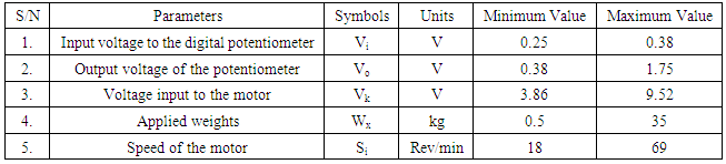
The dynamic parameters of the electromechanical motor system are listed in Table 2 with their respective minimum and maximum values. The data for the following dynamic parameters have been collected for this work:

1). The input voltage to the digital potentiometer; V_i;

2). The output voltage of the potentiometer in response to changes in the input; V_j;

3). The actual voltage input to the motor; V_k;

4). The input standards weights, W_x; and

5). The corresponding measured speed of the motor (in revolution per minute) in response to the changes in the inputs (voltage and applied weights). S_i.

The data were collected using three digital voltmeters connected simultaneously to measure the input voltage to the digital potentiometers (V_i), the output voltage of the potentiometer (V_j) and the actual voltage applied to the motor (V_k) respectively and this was maintained throughout the period of experimentation. Standard weights available in the laboratory ranging from 0.5 kg to 10 kg were combined to form a range of the applied weights from 0.5 kg to 35 kg. These were used as the applied weights or disturbances to the electromechanical system. More weights could be accommodated if the diameter of the container is increased and it will require replacement of the bowl and also change the design of the experimental system.

3.1. Data Measurement Procedure

With the complete system setup and the digital voltmeters connected, the system is powered firstly without applying any of the weights (no load condition) on the system and the input voltage (V_i) to the digital potentiometer measured with the first voltmeter, the output voltage (V_j) of the digital potentiometer measured with a second voltmeter, the voltage applied to the motor (V_k) measured with the third voltmeter and the speed S_i of the motor in revolution per minute was measured. Then the input voltage V_i was varied and the respective readings; V_j, V_k and S_i were recorded. For different input voltage to the digital potentiometer V_i, we measured and recorded the corresponding V_j, V_k and S_i without any weight. Subsequently, the weights are applied from 0.5 kg to 35 kg and the input voltage to the digital potentiometer V_i is varied through the same ranges for each of the weights W_i ; the respective V_j, V_k and S_i measurements were recorded which give a successive over 500 data collected.

The speed of the motor is affected by two parameters, namely: the input voltage V_k and the applied weights W_x. The data is presented in the Fig. 6(a), (b) and (c) and Fig. 7(a) and (b). The Fig. 6 (a), (b) and (c) show the digital pot input voltage, digital pot output voltage and the motor input voltage respectively. Fig. 7(a) and (b) show the revolution per minute and the applied weight respectively. The input voltage to the digital potentiometer spans from 0 V to 5 V and is assuming to be coming from the computer system where the controller is designed and implemented. The minimum measured voltage is 0.25 V and the maximum used for this research is 2.12 V. The output voltage from the digital potentiometer as measured spans from 0.38 V – 1.27 V. As the input digital voltage gradually increased, the output digital voltage also increased proportionately for the number of runs as presented in Fig. 7(a) and (b).

The PMDC PORCHE PPWPM432 motor input voltage is a controlled output voltage from the digital potentiometer which has been amplified using the rail-to-rail amplifier OP284 to give supply to the motor. As the input digital voltage is increased, the supply DC motor voltage also increased correspondingly as it spans from 3.86 V as measured to 8.37 V and is presented in Fig. 6 (c).

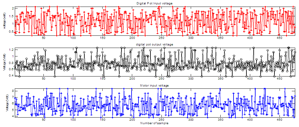Figure 6. Experimental data (a) Digital potentiometer input voltage, (b) Digital potentiometer output voltage and (c) Motor input voltage

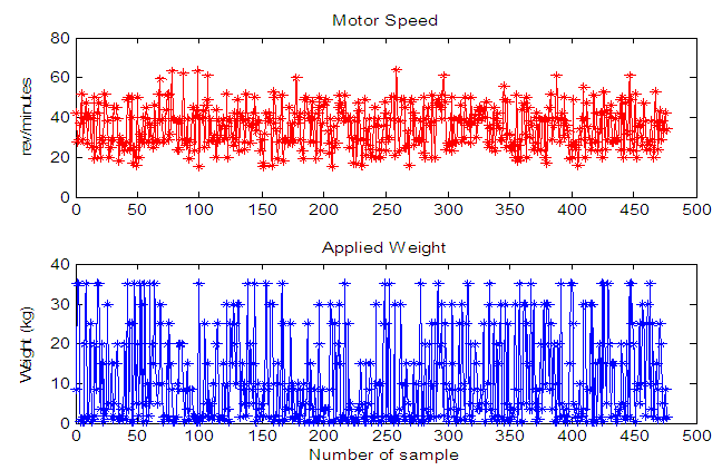Figure 7. Experimental data (a) motor speed (revolutions per minute) and (b) applied standard weights

Table 2. The dynamics parameters of the electromechanical system based on experimental measurements

3.2. Description of the Electromechanical System Input-Output Data

The picture of the designed and constructed electromechanical system, the front view and the interior view is presented in Fig. 8(a) and (b) respectively. The graph of the weights for the number of runs is presented in Fig. 6(b). The weights are combined to give a range from 0.5 kg to 35 kg limited by the diameter of the bowl on the iron plate. The speed of the system as measured by the counter circuit is presented in Fig. 6(a) the voltages were first fixed for no load condition; the speed in revolution per minute was recorded. Then the experiment was repeated for each of the applied weights keeping the voltages fixed and the respective revolution per minute as displayed by the counter recorded. The minimum recorded revolution per minute with no load is 18rev/minute while with 35 kg applied weight the counter recorded 15 rev/minute. The maximum speed recorded is 64 rev/ minute which occur at the highest supplied voltage and with no load but 51 rev/min with 35 kg weight applied.

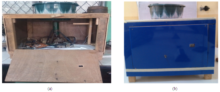Figure 8. Picture of the designed electromechanical speed control system (a) interior view and (b) completely cased system

The speed of the system in revolution per minute which is the output of the system is affected by two major parameters; the input voltage and the applied weights. The higher the input voltage, the faster the motor moved and the higher the weight applied the slower the system moved.

3.3. Effects of the Process Variables on the System

3.3.1. Disturbances

Disturbances are variables that fluctuate and cause the process output to move from the desired operating value (setpoint). A disturbance could be a change in flow or temperature of the surroundings or pressure etc. Disturbance variables can normally be further classified in terms of measured or unmeasured signals. The different weights applied (kg) in this research serve as the disturbance introduced to the system for the study and it ranges from 0.5 kg to 35 kg. More weights could be accommodated for further studies but the diameter of the bowl would need to be increased and the total design of the system would require adjustment.

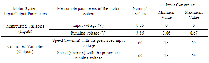
3.3.2. The Manipulated and Controlled Variables

The manipulated variable (MV) is the variable chosen to affect control over an output variable. As the output is being controlled it is normally referred to as the controlled variable (CV). The objective of a control system is to keep the CVs at their desired values (or setpoints). This is achieved by manipulating the MVs using a control algorithm. (Willis, 1999). The manipulated variables with the nominal values and constraints as well as the controlled variable with the nominal values and the constraints are as shown in Table 3. The manipulated variables are the input voltage to the digital potentiometer and the running voltage of the motor with nominal values of 0.25 V and 4.86 V respectively. The controlled variable is the output revolution per minutes of the motor with nominal value of 60 rev/min.

3.4. Desired Reference Trajectory for the Optimal Control of the Electromechanical Motor System

The main control objective for the electro-mechanical system in this research work is to maintain a revolution of the permanent magnet direct current (PMDC) reference at 60 revolutions per minute despite disturbances and its effects by manipulating the motors input voltage to stabilize the speed. The desired reference trajectory for the speed of the PMDC motor of the electro-mechanical system is illustrated in Fig. 9 and are described below as follows:

1). It is assumed that the system is turned on with the rotor, starting from the state of rest (0) then gradually increases in speed.

2). As the speed increases the voltage supply to the motor increases also to attain the 60 revolution per minute.

3). In the presence of disturbance the motors voltage is manipulated to keep the motor speed at the desired 60 revolution per minute

4). The process continues till the system is shutdown, then it gradually comes down to state of rest.

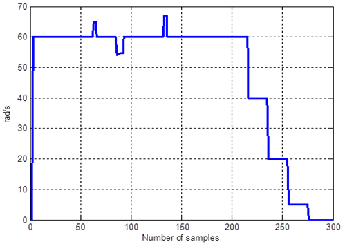Figure 9. The desired reference trajectory for the speed of the PMDC motor of the electromechanical motor system

3.5. Considerations of the Electromechanical System Speed Operations

The diagram for the practical implementation of the speed control system is shown in Fig. 10. Pulse width modulation (PWM) is generated through the digital potentiometer controlled circuit to drive the system and the output speed of the motor y(k) measured is encoded to be fed back to the summer which compares the feedback signal with the preset reference signal R(k) to determine the error ε(k) that would be adjusted by the controller to produce a new control input u(k) to the motor system which is used to control the motor system to follow the reference input. However, to control any system in this way, the model of the system is required hence the model of the motor system is obtained and used as a feedback into the controller. The controller unit as well as the model of the motor and the encoder is all supposedly located on a personal computer (PC) system which is interfaced to the motor system.

Table 3. Manipulated variables (MV) and the controlled variables (CV) with the motor system constraints

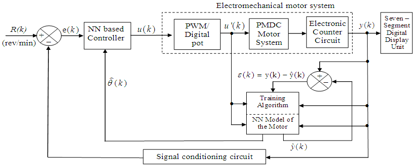Figure 10. Block diagram for the practical implementation of the adaptive speed control system for the electromechanical motor system

4. Conclusions and Future Direction

The design and construction of an electromechanical permanent magnet direct current (PMDC motor system using PORCHE PPWPM432 electric motor have been carefully presented as well as a novel technique on how the proposed design could be adopted for the formulation and design of an adaptive speed control problem. Furthermore, the technique for data acquisition from the designed and constructed electromechanical motor system have been detailed which can be employed for real-time online system identification and adaptive control of the proposed system.

If properly designed and implemented, the proposed system identification and adaptive control scheme could override existing techniques in literature since it does not require the actual mathematical modeling of the electromechanical motor system but rather depends only on the actuator (input) and sensor (output) data measurements for dynamic modeling and adaptive control. As a future work, it may be necessary to formulate and design an adaptive control that could employ the input and output data measurements directly for the dynamic modeling and adaptive control of the electromechanical motor system in the context of adaptive speed control systems design.

It is also worthy to note that the design of adaptive controllers for speed control of electromechanical systems with relative short sampling time have proven unsuccessful when implemented on multipurpose personal computer, microprocessor, microcontroller as well as on low-end embedded systems (Elmas and Ustun, 2008). Thus, the employment of high-end embedded systems such as complex programmable logic devices (CPLDs), field programmable gate arrays (FPGAs), application specific integrated circuits (ASICs), etc for the implementation of dynamic modeling and adaptive control algorithms for the electromechanical motor system is recommended and could be considered as a future direction for adaptive speed control systems design.