1. Introduction

There are many models presented in time series literature for forecasting problem. Traditional models may fail to satisfy to analyze many data sets which have various assumptions. From this point of view, especially over the last decades, artificial neural networks (ANNs) that do not include such strict assumptions have been widely taken advantage of as an alternative forecasting approach. The most important characteristic of ANN is that it has the ability to learn from a source of information (data). Learning process of ANN is the process of getting the best values of weights and this process is called as the training of ANN. The training problem of ANN can be regarded as an optimization problem. In the literature, although Levenberg-Marquardt and Back Propagation (BP) learning algorithms have been used to train ANN, some heuristic algorithms such as genetic algorithms, particle swarm optimization, differential evolution algorithm, simulated annealing and taboo search algorithm are also used, to train ANN especially in recent years.

The first ANN model was proposed by [1]. Multilayer perceptron (MLP) was presented by [2] in order to solve a non-linear problem. A MLP model is composed of an input and output, and one or more hidden layer(s). Various ANN models were put forward by [3-6]. Moreover generalized mean neuron model (GMN) and geometric mean neuron (G-MN) model were introduced by [7, 8], respectively. [9] presented an approach to get combining forecast by using ANN. In time series forecasting problem, multi-layer feed forward artificial neural networks (ML-FF-ANN) model have been most commonly used. The time series forecasting literature based on ANN was summarized by [10]. And also [11-14], for forecasting real-world time series, touched on the issue of network structure in their studies. Even though feed forward artificial neural networks can produce successful forecasting results, they have an architecture selection problem that can have a negative effect on the forecasting performance of ANN. Therefore the determination of the numbers of neurons in the layers in ML-FF- ANN is a crucial problem. [15] proposed single multiplicative neuron model artificial neural network (SMNM-ANN) that has a single neuron and does not have architecture selection problem. While [15] used back propagation learning algorithm, [16] used cooperative random particle swarm optimization (CRPSO) in the learning process of SMNM-ANN. And also, the modified particle swarm optimization method and differential evolution algorithm (DEA) were utilized to train MNM-ANN by [17, 18].

In this study, bat algorithm (BA) that is used in new studies frequently is firstly utilized for the training of SMNM-ANN in time series forecasting. BA is based on the echolocation features of micro-bats (Yang, 2010) and bats are very good at finding the prey. They can distinguish very small prey and obstacles even in the dark. The algorithm mimics the same process of how bats can find and detect the food source with the help of echolocation. To support the idea that SMNM-ANN trained by BA (BA-SMNM-ANN) has satisfied forecasting performance, two well-known real-life time series data were analyzed. Section 2 gives an introduction of BA-SMNM-ANN and an algorithm of training process. The implementation and the obtained results are presented in Section 3. And finally last section provides some discussions.

2. The Proposed Method

There are various studies that show SMNM-ANN is effectively used in time series forecasting. Different learning algorithms have been used in the training process of SMNM-ANN to get better forecasting results.

In this study, SMNM-ANN is firstly trained by BA. Since the proposed BA-SMNM-ANN model is basically a SMNM, it has same structure with SMNM and it can be demonstrated in Figure 1.

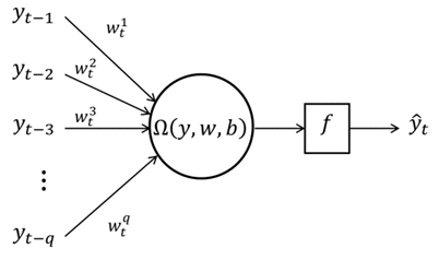Figure 1. The structure of a BA-SMNM-ANN

In Figure 1, function is the product of the weighted inputs and also shows the activation function. Here, 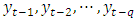and are inputs and outputs of BA-SMNM-ANN, respectively. Moreover, q can be called as model order, n is the number of observations in training set of time series. The SMNM-ANN with q inputs given in Figure 1 has weights. Of these, q are the weights corresponding to the inputs 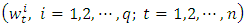and q to the sides of the weights 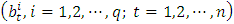. The optimization process can be also called as the training of BA-SMNM-ANN. The weights and biases are shown with and . Thus, each member of bat population has positions. The structure of a member of bat population is illustrated in Figure 2.

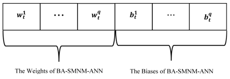Figure 2. The structure of a bat

The algorithm of BA-SMNM-ANN is given steps by steps as below.

Step 1. Generate a set of bat population

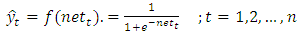
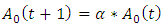
Velocities , positions , rate , and loudness are generated. The initial values of and and are constant parameters.

Step 2. Calculate the fitness value of each bat in the population.

To obtain fitness function values, firstly the outputs of the network are calculated by using following equations;

(1)

(2)

And also, root mean square error (RMSE) is calculated as the fitness function value;

(3)

Step 3. Update variables for bats flying randomly

Following steps are applied for each bat.

Step 3.1. Generate from uniform distribution with parameters.

Step 3.2. Calculate velocities and positions of bats by using following formula.

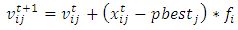(4)

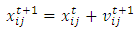(5)

Step 3.3. is generated from uniform distribution with the parameters . If , positions of bats are updated by using following formula.

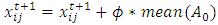(6)

In this Equation, is a random number and it is generated from uniform distribution with the parameters . Besides, is a vector and its elements are constituted by average loudness of all bats.

Step 3.4. is generated from uniform distribution with the parameters . If and new fitness value of the bat is smaller than the previous fitness value of the bat at the same time.

(7)

(8)

Pbest is updated. Otherwise .

Step 4. Check the stopping criteria.

If it is reached to the maximum number of iterations or the fitness value calculated from the bat population with the best fitness value. is less than a predetermined value the process is end, otherwise move to Step 3.

3. Implementation

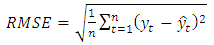
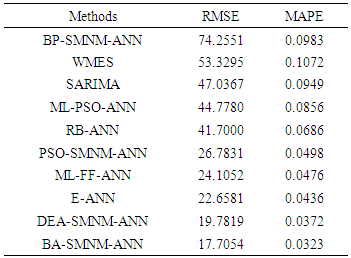
To show the performance of the BA-SMNM-ANN, Australian Beer Consumption “(AUST)" data with 148 observations between years 1956 and 1994 was analyzed firstly.

The results obtained from various methods have been compared in respect to RMSE and Mean Absolute Percentage Error (MAPE) criteria given in Eq. 7.

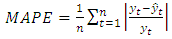(9)

In this Equation, and show the number of training samples, observed values and the forecasting values, respectively.

The last 16 observations of the time series was taken as test data. In addition to the proposed method, AUST data, given in Figure 3, was analyzed by seasonal autoregressive integrated moving average (SARIMA), Winter's multiplicative exponential smoothing (WMES), Multi-layer feed-forward neural network (ML-FF-ANN), Multilayer neural network based on particle swarm optimization (ML-PSO-ANN), Back propagation learning algorithm based on single multiplicative neuron model neural network (BP-SMNM-ANN), single multiplicative neuron model artificial neural network based on particle swarm optimization (PSO-SMNM-ANN), single multiplicative neuron model artificial neural network based on differential evolution algorithm (DA-SMNM-ANN), Radial basis artificial neural network (RB-ANN), Elman neural network (E-ANN) methods.

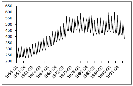Figure 3. AUST data between the years of 1956-1994

RMSE and MAPE criteria values for test set obtained from proposed model and other methods in the literature are given in Table 1.

Table 1. The results obtained from all methods for AUST data

With Table 1, we can clearly say that the proposed BA-SMNM-ANN has the best performance among all methods in terms of both RMSE and MAPE criteria.

Besides, the graph of the real observations and the forecasts obtained from proposed method for test set is given in Figure 4. According to this graph, it is obvious that the forecasts obtained from BA-SMNM-ANN are compatible with the real observations.

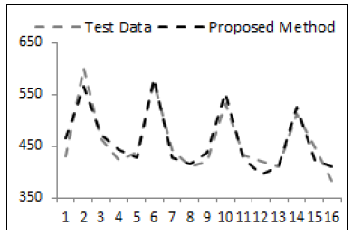Figure 4. The graph of real observations and forecasts obtained from proposed method for AUST data

Finally, the proposed method was analyzed for Canadian lynx data between years 1821 and 1934. The last 14 observations of the time series was taken as test data. The logarithm (to the base 10) of the data was used in the analysis. The graph of the Canadian logarithmic lynx data is given in Figure 5.

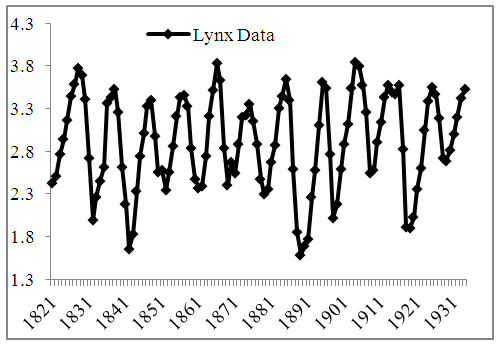Figure 5. Logarithmic Canadian lynx data series (1821-1934)

This data set was also analyzed with SARIMA, WMES, RB-ANN, ML-FF-ANN, BP-SMNM-ANN, autoregressive integrated moving average (ARIMA), PSO-SMNM-ANN and [19]. During the analysis of Canadian lynx data, the model orders in other words the number of inputs of BA-SMNM-ANN (m) was changed from 2 to 4. The number of positions (np) in the population was changed from 30 to 100. The number of iteration was determined as 100.

At the end of the analysis, we conclude that the best result is obtained in the case where m=4, np=30.

In addition, MAPE criteria values for test set obtained from proposed method and other methods in the literature were given in Table 2.

Table 2. The forecasting results obtained from the proposed method for Logarithmic Canadian Lynx Data

With Table 2, we can clearly say that the proposed BA-SMNM-ANN has the best performance among all methods in terms MAPE criteria.

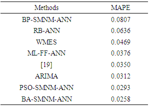
4. Discussion and Conclusions

Several kind of ANN model is used in time series forecasting literature. Although ML-FF-ANN has been commonly used in the forecasting problem of time series, the architecture selection problem of it is crucial to get the reasonable forecasts. SMNM-ANN has not also such a problem because it has only one neuron. To train SMNM-ANN, there are various learning algorithms in the literature.

In this paper, for time series forecasting problems, SMNM-ANN is trained by BA. By favour of real-life time series implementations, the outstanding forecasting performance of BA-SMNM-ANN has been brought to light.