Uduak Idio Akpan 1, Uduak Etim Udoka 2, E. H. Johnson 1
1Department of Elect/Elect Engineering, Akwa Ibom State University, Ikot Akpaden, Nigeria
2Department of Elect/Elect and Computer Engineering, University of Uyo, Uyo, Nigeria
Correspondence to: Uduak Idio Akpan , Department of Elect/Elect Engineering, Akwa Ibom State University, Ikot Akpaden, Nigeria.
| Email: |  |
Copyright © 2016 Scientific & Academic Publishing. All Rights Reserved.
This work is licensed under the Creative Commons Attribution International License (CC BY).
http://creativecommons.org/licenses/by/4.0/

Abstract
Enhanced Interior Gateway Routing Protocol (EIGRP) is one of the hybrid protocols, which is based on Interior Gateway Routing Protocol (IGRP). EIGRP has the ability to scale to an enterprise network size, not quite as large as an OSPF network can scale but a lot larger than a network running RIP can handle. In this paper, a new shortest path first algorithm used in enhanced interior gateway routing protocol (EIGRP) is proposed. The problems associated with existing protocol were identified and a new shortest path algorithm was developed to address the end-to-end delay problem. Mathematical expressions were developed to quantitatively represent the performance of the proposed algorithm. We carried out analysis on the performance of the proposed algorithm. In all, the new algorithm has a smaller end-to-end delay when compared to that of the existing shortest path algorithm used in EIGRP routing protocol.
Keywords:
Routing protocol, Delay metrics, VOIP
Cite this paper: Uduak Idio Akpan , Uduak Etim Udoka , E. H. Johnson , Improved Shortest Path First Algorithm for Enhanced Interior Gateway Routing Protocol (EIGRP), American Journal of Intelligent Systems, Vol. 6 No. 2, 2016, pp. 31-41. doi: 10.5923/j.ajis.20160602.01.
1. Introduction
Voice over Internet Protocol (VoIP) technology has offered cost-saving solution for integrated data and voice network (IDVN). This has taken off as a viable alternative to the traditional voice systems and the Public Switched Telephone Networks (PSTN). VoIP in essence is flexible in driving new services by optimising the device interoperability using standards-based protocols. When designing a network to support VoIP and real-time applications, certain considerations such as application requirements, available budget, quality of service requirements, and downtime ramifications, have to be taken into account. Some approaches have been seen to support VoIP service effectively. A notable and reliable of these approaches is the best effort network design (BEND). VoIP is a real-time application and consequently provides new challenges for service providers and enterprises. Therefore, networks need to be more intelligent, secure, and should have a higher level of performance. The challenges in the deployment of VOIP are enormous. Some of these include.
1.1. Interoperability
The biggest challenge for network managers to overcome is the multi-vendor interoperability. There are a few important VoIP protocol stacks which have been defined by various standard bodies and vendors, namely H.323, Session Initiation Protocol (SIP) and Media Gateway Control Protocol (MGCP). While the ITU-T’s recommendation (H.323) is gaining wide recognition, many vendors are yet to completely comply with all the guidelines and other recommendations. As the result of this, the technologies and equipment for implementing complete VoIP networks are still not operational at a feasible level.
1.2. Security
Security has been seen as a major concern in VoIP networks. Although H.323 defines encryption and authentication of user access, hackers can still tap into any conversation on the system, which means an employee or any outsider with internet access can monitor the voice conversations without ever having to leave the desk [1]. Another security challenge can arise if a corporation uses VoIP technology for a remote access location. This however is one of the main uses for partial VoIP implementation today and often involves issues with firewalls. For instance, the H.323 requires direct access to the company network and will open the entire network up to all UDP and TCP traffic. To solve this challenge, all H.323 traffic should be contained within one region and a voice trunk then used to connect traffic between the isolated region and the rest of the network. Another viable solution is to use an H.323-aware firewall.
1.3. Bandwidth Management
Also considered as a major challenge in VOIP is lack of bandwidth management of current networks employed within most large corporations. VoIP generates two types of network traffic – the control messages, and the digitally encoded voice conversations. The control messages are used to setup and manage connections between IP phones and an IP PBX. The involved protocols normally use very little bandwidth and a delay of a few seconds in setting up a call is usually acceptable [2]. The real challenge however is to satisfy the bandwidth demands of the digitized voice streams between users. Each conversation consumes nearly constant amount of bandwidth for the duration of the call. The bandwidth required for each call depends primarily on the voice encoding technique as well as a couple of other variables. Two voice encoding standards widely supported by VoIP products are G.711 and G.729. Interestingly, there is problem of incompatibility with the codecs from different vendors. The bandwidth requirements for large companies or Universities for instance, are much larger than for small companies and departments. Because the codec is the required components for converting analogue waves into packets of digital signals, the frame relays of large companies are over taxed. Slower and more taxing working systems demand greater bandwidth for the codec. The reliance of large-scale implementation of VoIP technology is a big challenge for large corporations at the present time.
2. Interior Gateway Protocols (IGP)
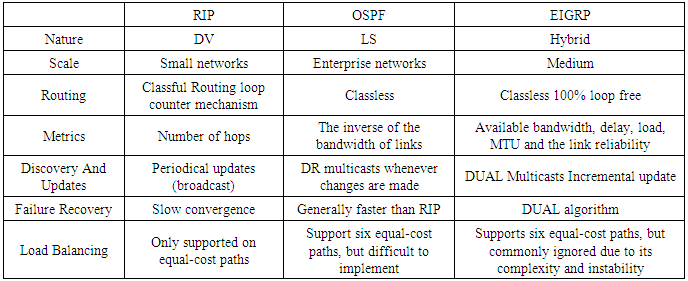
Dynamic routing protocols fall into three categories: Distance Vector (DV), Link State (LS) and hybrid protocols. The knowledge information shared by different network segments is defined by the routing protocol selected, which are stored in routing tables. To maintain an up-to-date routing table the router must determine the best information to be stored. Each protocol determines this based on a certain criterion with the use of algorithms, which compile values known as metrics. Metrics are generated from as little as one characteristics of the network or more often several characteristics. The most common measurements normally include hop counts, delay, bandwidth, load, reliability (i.e. errors on the link), cost, etc. Among the three types of routing protocols, the simplest to configure is the distance vector protocol which use the distance and direction to find the best path to the destination by using an algorithm called the Bellman-Ford algorithm. Network discovery is achieved by gathering information from directly connected neighbouring routers which in turn may have gained their information from neighbouring routers. To share this information distance vector protocols use a method known as a local broadcast. This sends out data to any device that is connected to an interface of the router. Distance vector does not care who receives and processes these broadcasts and that they are periodic in their approach [1]. These protocols will send out updates at regular intervals regardless of whether or not there is a topology change. As these packets regularly traverse the network, a large amount of unwanted network traffic, can be generated. Examples of distance vector protocols are RIPv1, IGRP, etc.
2.1. RIP Version 1
RIP version1 is a DV routing protocol that is easy to comprehend and deploy within an AS. Although superseded by more complex routing algorithms, RIP is still widely used in smaller ASs due to its simplicity. RIP makes no formal distinction between networks and hosts. Routers typically provide a gateway for datagram to leave one network or AS and to be forwarded onward to another network. Routers therefore, have to make decisions if there is a choice of forwarding path on offer. The metric system RIP networks use is the hop count, which has a maximum value of 15 or 16 [4]. Every time a router passes the routing table to other routers a value of 1 is added to the metric inside the routing update. The maximum number of hop count is to solve the routing loops problem. Routing loops are basically confusions in a network topology that occur when the update/age out timers can be inefficient. With the hop count set to 15 the packet can be passed through a maximum of 15 routers before being discarded, without which the packets can be passed indefinitely until either the network crashes or the routers are switched off. RIP supports up to a maximum of 6 equal-cost path to a destination, this means that is a destination is reachable over different routes that have the same amount of hops, the router will hold all routes in memory up to a maximum of six (four is the default) [1]. The paths are all placed into the routers table and can be used to load balance when sending data. The main features of RIP can also lead to its disadvantages, such as information flooding, ineffectiveness of metrics system, and classful routing algorithm.
2.2. Open Shortest Path First
Open Shortest Path First (OSPF) is based on open standards and has good compatibility on a wider range of equipment, which is a prevalent routing protocol in larger enterprise networks. It is a LS routing protocol which uses more complex metric system to give efficient pathways discovery solutions to remote networks. The cost to measure the metric is worked out by taking the inverse of the bandwidth of links. Essentially a faster link is lower in cost. The lowest cost paths to remote networks are the most preferred routes, and held in the routing table. OSPF can load balance across a maximum of six equal-cost path links, although doing this can cause difficulties. The serial interface of the router is configured with a clock rate and a bandwidth. The clock rate is the speed that data can be sent across a link, and the bandwidth is used by the routing protocol in the metric calculations. By default the speed of a serial interface is set to 1544 Kbps [2]. There is a potential hazard of this system. When different clock rates are set on a different link, the bandwidth has to be accordingly configured; otherwise OSPF will regard both connections as the same speed, which will cause problem with load balancing [3]. When routers need to run OSPF frequently, lots of resources are dedicated to the process; this potential problem can dramatically slow down the network service speed.There are some major differences between OSPF and RIP. Firstly, comparing to RIP, OSPF is a classless protocol which allows utilization of different subnet masks, which essentially gives network administrators more flexibility with IP addresses and less wastage. Secondly, one appealing advantage that OSPF offers over RIP is scalability. OSPF has the knowledge of ASs and areas, and is able to understand the hierarchical routing structure. Thirdly, as a LS protocol, OSPF only sends out update information when there is a change in the network, rather than sending periodic updates at regular intervals as in DV protocols. This quality saves the bandwidth utilization throughout the entire network communications. Fourthly, while RIP uses broadcast to pass on routing information throughout networks which can cause potential network congestion problems, OSPF uses multicast method to reduce network traffic which uses addresses that are destined for particular machines. [2] [7] [9]
2.3. Enhanced Interior Gateway Routing Protocol (EIGRP)
Enhanced Interior Gateway Routing Protocol (EIGRP) is one of the hybrid protocols, which is based on Interior Gateway Routing Protocol (IGRP). EIGRP has the ability to scale to an enterprise network size, not quite as large as an OSPF network can scale but a lot larger than a network running RIP can handle. EIGRP calculates distance by using a collaboration of different information. The characteristics selected are available bandwidth, delay, load, maximum transmission unit (MTU) and the link reliability. By using these factors the selected paths can be finely tuned, so information can be passed around a network by the faster most reliable routes. By default only bandwidth and delay are used. EIGRP is also a classless protocol and will support load balancing across six unequal paths. This however is not such a simple command to use, and requires manual configuration. If incorrectly configured, it can cause network instability and routing loops, hence it is a common practice to ignore this ability [17].
2.4. Summary of Comparisons
Based on the above discussions, the comparisons of the three routing protocols are summarized in Table 1.Table 1. Comparison of RIP, OSPF and EIGRP
 |
| |
|
3. Methodology
This research adopts the EIGRP bandwidth estimation and routing path selection model.
3.1. Description of the EIGRP Bandwidth Estimation and Routing Path Selection
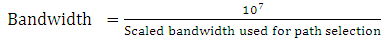
EIGRP defines the bandwidth of a path as the minimum of the residual bandwidth of all links on the path or the bottleneck bandwidth. Typically, in EIGRP, two delay metrics are considered. These are: propagation delay and queuing delay. The queuing delay is considered to be closely related to the bottleneck bandwidth and traffic characteristics. In order to avoid inter-dependence among the identified delay metrics, only the propagation delay is used in the delay metric. This helps to simplify and modify the delay path computation [16] [17] [19].EIGRP in principles adds weighted values of different network link characteristics together in order to calculate a metric for routing path selection. These characteristics include:i. Delay (measured in of microseconds)ii. Bandwidth (measured in kilobytes per second)iii. Reliability (in numbers ranging from 1 to 255; 255 being the most reliable)iv. Load (in numbers ranging from 1 to 255; 255 being considered saturated)Since, EIGRP calculates the total metric by scaling the bandwidth and delay metrics, we consider BW(i) to be the scaled bandwidth for outgoing interface i. Also, EIGRP uses the following formula to scale the bandwidth;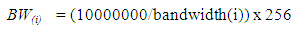 | (1) |
If we consider  to be the minimum scaled bandwidth for outgoing interface i, then;We can say
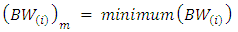 | (2) |
where  is the least bandwidth of all outgoing interfaces on the router to the destination network usually represented in kilobits.To scale the delay, EIGRP model considers the formula
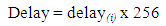 | (3) |
where delay(i) is the sum of the delays configured on the interfaces, on the router to the destination network, in tens of microseconds. EIGRP Total Delay Metric (EIGRPTDM) is derived from the EIGRP scaled values as | (4) |
Various user-defined constants, K1 through K5, normally set by the user to produce varying routing behaviours. However, by default, only delay and bandwidth are used in the weighted formula to produce a single 32-bit metric. These values of K should be used after careful planning. Failure of the network convergence occurs on the account of mismatched values of K by preventing neighbour relationships. If K5 = 0, Then,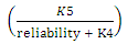 | (5) |
The  formula becomes;
 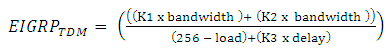 | (6) |
The default values for the various values of K are;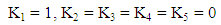 | (7) |
By default, the  can be simplified further as
  | (8) |
 | (9) |
If we consider the effective bandwidth for path selection in the existing EIGRP protocol as BandwidthExistingAlg, from equations 9 and 2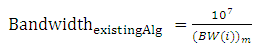 | (10) |
Since the values are configured manually on the router interfaces, the expected delay on an interface and the needed bandwidth on a link are configured to suit the network needs. In other to obtain the total delay along each path, the delays at each hop are summed. The summed delay is the link delay and is usually used by the protocol for metric calculation. However, this delay comprised processing delay, propagation delay, transmission delay and queuing delay. Hence, the total delay, (Dt) can be expressed as follows;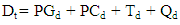 | (11) |
Where, PGd is the propagation delay, PCd is the processing delay, Td is the transmission delay and Qd is the queuing delayTherefore, 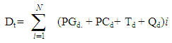 | (12) |
The Queuing Delay, Qd is given as: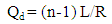 | (13) |
Where L and R are packet size and transmission rate respectively.It is worthy to note that, queuing delay is the length of time a packet waits in the interface queue before being sent to the transmit ring. Queuing delay depends on the number and size of packets in the queue, and the queuing methods used. The Transmission delay, Td is given as, | (14) |
Transmission delay is the time between the transmission of the first bit and last bit of the packet. If the packet size is fixed, the time is a constant. The Propagation Delay, PGd is given as: | (15) |
Where m and s denote link distance and link speed respectively.Propagation Delay is the length of time it takes the packet to move from one end of the link to the other. Propagation delay depends on the type of media, such as fiber or satellite links. The Processing Delay, PCd is given as: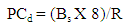 | (16) |
Where Bs and R denote file size to be transmitted and transmission rate respectively.Processing Delay is the time it takes a packet to move from the input interface of a router or Layer 3 switch, to the output interface. Processing delay depends on switching mode, CPU speed and utilization, the router’s architecture, and interface configuration and is given by;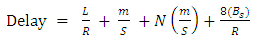 | (17) |
Let  for the existing EIGRP be EIGRPTDMExisting, therefore from equations 7, 9, 11, 12, 13, 14 and 15, 16 and 17
  | (18) |
L = packet size, R = transmission rate/link Bw, N = number of nodes, M = link distance, S = link speed and Bs = file size to be transmitted.In a network with many routes, EIGRP chooses the path with least metric.
3.2. Description of the New Shortest Path Algorithm for EIGRP
The EIGRP uses minimum link bandwidth to determine the shortest path and hence to select the routing path. However, using only the minimum bandwidth deprives the path of its optimal metric values. Therefore, to obtain optimal metric values, we consider, in this research average bandwidth across a path. This as would be proven has a great a great influence in the metric. We consider (BWi)avg as the average of all the scaled bandwidth for outgoing interfaces, i, n as the number of outgoing interfaces, and  as the scaled bandwidth for outgoing interface, i, as given in equation 1
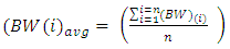 | (19) |
Proposed algorithm for EIGRP uses, (BWi)avg (that is the average of all the scaled bandwidth for outgoing interface, i,) for its path selection. Next, let the effective bandwidth used for path selection in the proposed algorithm for EIGRP protocol be  , then from equations 8 and 18
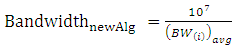 | (20) |
Let  for the new algorithm for EIGRP be defined as
  then, from equation 7
 | (21) |
Then, substituting equation 18 for delay in equation 21 gives; 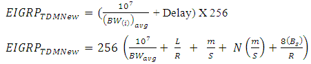 | (22) |
Finally, from the foregoing analysis, the existing shortest path algorithm used in EIGRP routing protocol uses  of Equation 18 the for its path selection.
  is computed based on the value of
  , that is, the minimum scaled bandwidth for all the outgoing interface in the router. On the other hand, the new shortest path algorithm proposed in this research for EIGRP routing protocol uses
  of equation 22 for its path selection.
 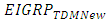 is computed based on the value of
  , that is, the average of all then scaled bandwidth for all the outgoing interface in the router.Figures 1 and 2 are the sample network configurations for comparative analysis of performance of the existing shortest path algorithm used in EIGRP and new shortest path algorithm proposed in this paper for EIGRP routing protocol.
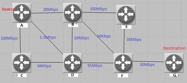 | Figure 1. Simple Network Configuration for Comparative Analysis of the New and Existing Algorithms for EIGRP |
 | Figure 2. Complex Network Configurations for Comparative Analysis of the New and Existing Algorithms for EIGRP |
4. Results and Discussion
The results of the analysis on the proposed EIGRP routing protocol is presented in this section.
4.1. System Parameters
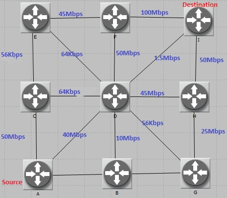
This section presents the parameters and their values for the computation of the results. Table 1 details the different paths through which data can be transmitted from source to destination. It also shows minimum bandwidth along each path and the computed average link bandwidths. The different bandwidths are used to calculate EIGRP metrics for selecting the best path. It is assume that a data of size 10Kb is to be transmitted from source to destination as shown in the table 2.Table 2. Different paths in the network and their corresponding link bandwidths
 |
| |
|
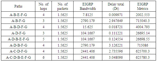
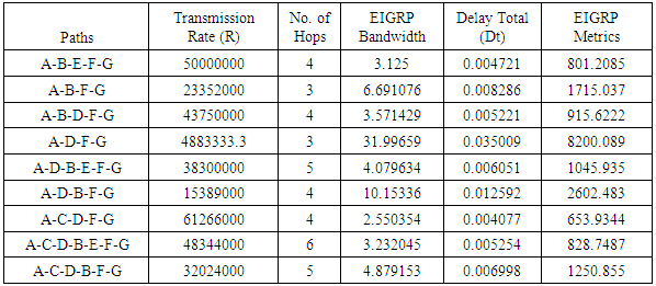
Table 2 shows the computed delay and Metrics of the different paths calculated using minimum link bandwidth. From the table it can be deduced that the path with the minimum Metric is path A-B-E-F-G with minimum metric value of 2002.553 which is truncated to 2002. This implies that protocol will choose the path through A-B-E-F-G for routing packets.The metric for the new shortest path algorithm for EIGRP which uses average link bandwidth is also given in Table 2.Table 3 shows the computed delay and Metrics of the different paths calculated using the new formula (average link bandwidth). From the table it is observed that the path with the minimum Metric is path A-C-D-F-G with minimum metric value of 653.9344 which is truncated to 653. This implies that the protocol will choose the path through A-C-D-F-G for routing packets. It can be deduced from the two scenarios that different paths were chosen by EIGRP for routing packets across the network. Furthermore, it is observed that the Metric values for both the existing and new formula are not the same; while the minimum metric for the existing formula is 2002, that of the new formula is 653 which is far smaller compared to the old metric.Table 3. Computed Metrics for existing shortest path algorithm for EIGRP
 |
| |
|
Also noticed was the fact the delay difference in both cases. It takes longer time to route packets from source to destination using the old formula than the new one; meaning that the new formula also improve delay.Table 4 identifies the different paths and their corresponding minimum link bandwidth and average path bandwidths.Table 4. Computed Metrics for the new shortest path algorithm for EIGRP
 |
| |
|
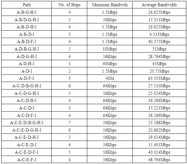
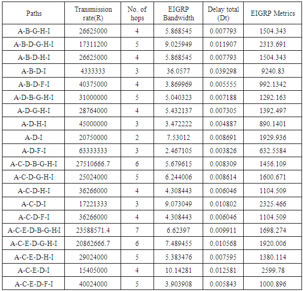
Table 4 identifies the diverse paths in the network through which packets can be transmitted from source to destination and their corresponding minimum link bandwidth and computed average path bandwidths. It also highlights the number of hops along each path from source to destination. The different bandwidths are used to calculate EIGRP metrics for selecting the best path. It is assume that a data of size 10Kb is to be transmitted from source to destination as shown in the Table 5.Table 5. Different paths in the network and their corresponding link bandwidths
 |
| |
|
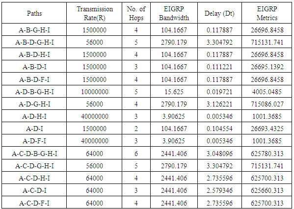
Table 5 shows the computed delay and Metrics of the different paths calculated using minimum link bandwidth. From the table it can be observed that two paths have the same delay and minimum bandwidth metric value. The routes through A-D-H-I and A-D-F-I have equal delay value of 0.005346and equal metric value of 1001.3685. This implies that the protocol will choose the path through any of these two links with equal metric or may divide the packets through both paths.Table 6 shows the computed delay and Metrics of the different paths calculated using the new algorithm (average path bandwidth). From the table it can be observed that only one path has a minimum metric 632.5584 as opposed to that of the existing algorithm which saw two paths with same delay and minimum bandwidth metric value. The routes through A-D-H-I is the path with minimum bandwidth. This implies that EIGRP protocol will choose the path through A-D-H-I to transmit packets from source to destination. We can say that the new algorithm is more precise than the old algorithm as observed in the scenario treated above. It can also be observed that the values for both delays and metrics for the new algorithm is smaller compare to that of the old algorithm.Table 6. Calculated Metrics for existing shortest path algorithm for EIGRP
 |
| |
|
Table 7. Calculated Metrics for the new shortest path algorithm for EIGRP (with average link bandwidth)
 |
| |
|
Using the two formulas, we shall compute metric for different data sizes larger than 10Kb considered above and observe the degree of improvement of the new formula over the old formula.In figure 3, the effect of packets transmission rate on the total transmission delay for 4 hops is investigated. It is observed that the increase in the rate of transmission results in reduced total transmission delay. This can be explained from the fact that, as the rate of transmission is increased, more packets can be transmitted and the delay in transmission will be reduced.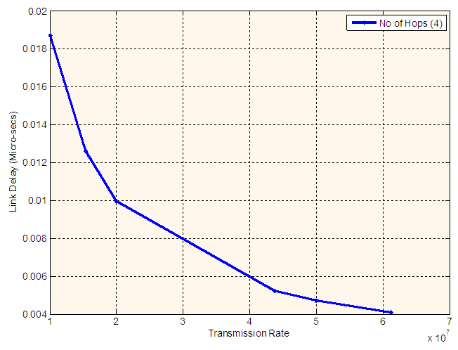 | Figure 3. Effect of Transmission Rate on Link Transmission Delay for four Hops |
In figure 4 the effect of packets transmission rate on the total transmission delay for 4 paths and 5 paths is investigated. It is observed that the increase in the rate of transmission results in reduced total transmission delay. This can be explained from the fact that, as the rate of transmission is increased, more packets can be transmitted and the delay in transmission will be reduced. Also noted is the fact that with the 5 paths, the delay is higher than that of 4 paths. This concludes that as the number of path increases, the more the total transmission delay.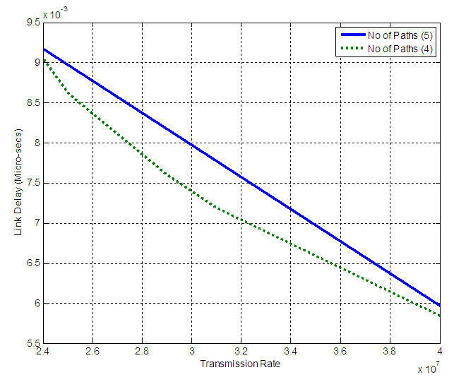 | Figure 4. Effect of transmission rate on link transmission delay for four and five hops |
Figure 5 depicts the effect of packet size on delay for the new algorithm. As the packet size increases, the transmission delay increases. It can be concluded that, a larger packet size take a higher time for transmission.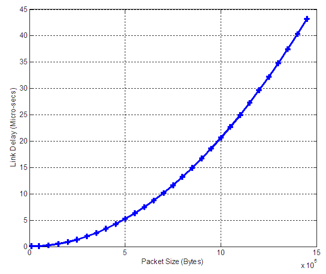 | Figure 5. Packet Size against Delay for the proposed Algorithm |
5. Conclusions
In this research, the existing shortest path algorithm used in EIGRP routing protocol was studied, problems were identified and a new shortest path algorithm was developed to address the identified problems. Specifically, the problem addressed in this research is on the end-to-end delay in the existing shortest path algorithm used in EIGRP routing protocol. Mathematical expressions were developed to quantitatively represent the performance of the existing shortest path algorithm used in EIGRP routing protocol. Then, a new shortest path algorithm was developed for EIGRP routing protocol. Mathematical expressions were developed to quantitatively represent the performance of the new algorithm. In all, the proposed algorithm has a smaller end-to-end delay when compared to that of the existing shortest path algorithm used in EIGRP routing protocol.
References
| [1] | M. Sportack, “IP Routing Fundamentals,” 2nd ed. California: Cisco Press. pp. 23, 1999. |
| [2] | T. F. Johansson, “Bandwidth efficient AMR Operation for VoIP,” IEEE Proceedings of the Workshop on Speech Coding, 3, 150-152, 2002. |
| [3] | C. Xianhui and J. C. Lee, “VoIP Performance over Different Interior Gateway Protocols,” International Journal of Communication Networks and Information Security (IJCNIS), 1 (1): 34-39, 2009. |
| [4] | J. C. Bolot, “Characterizing End-to-End Packet Delay and Loss in the Internet,” ACM SIGCOMM, 2(4): 289–98, 1993. |
| [5] | R. L. Carter, and M. E. Crovella, “Measuring Bottleneck Link Speed in Packet-Switched Networks,” Proc. Perf. Eval. 27(28): 297–318 1996. |
| [6] | M. Jain, and C. Dovrolis, “End-to-End Available Bandwidth: Measurement Methodology, Dynamics, and Relation with TCP Throughput,” ACM SIGCOMM., 34, 295–308, 2002. |
| [7] | A. M. Mark, “Voice over IP Technologies: Building the Converged Network,” 2nd ed. New York: John Wiley and Sons, Inc. pp. 234-237, 2002. |
| [8] | A. R. Nohl, and G. Molnar, “The convergence of the OSPF Routing Protocol,” Periodica Polytechnica Electrical Engineering, 47(1-2): 89-100, 2002. |
| [9] | M. Rashed, and M. Kabir, “A Comparative Study of Different Queuing Techniques in VOIP, Video Conferencing and File Transfer,” Daffodil International University Journal of Science and Technology, 5(1), 37-47, 2010. |
| [10] | S. G. Thorenoor, “Dynamic Routing Protocol Implementation Decision between EIGRP, OSPF and RIP Based on Technical Background using OPNET Modeler,” 2010 Second International Conference on Computer and Network Technology (ICCNT 2010), 191-195. |
| [11] | V. Paxson, “End-to-End Internet Packet Dynamics,” IEEE/ACM Trans. Net., 7 (3): 277-292, 1996. |
| [12] | K. Archana, S. Reena and A. Dayanand, “Performance Analysis of Routing Protocols for Real Time Application,” International Journal of Advanced Research in Computer and Communication Engineering. 3(1): 23- 25, 2014. |
| [13] | N. Hu and P. Steenkiste, “Evaluation and Characterization of Available Bandwidth Probing Techniques,” Proc. IEEE JSAC, 23, 789-791, 2003. |
| [14] | T. M. Jaafar, G. F. Riley, D. Reddy and D. Blair, “Simulation-Based Routing Protocol Performance Analysis: A Case Study,” 38th Conference on Winter Simulation, 234-240, 2006. |
| [15] | S. Floyd and T. Henderson, “The New Reno Modification to TCP’s Fast Recovery Algorithm,” RFC 2582. 2, 34-38, 1999. |
| [16] | S. Brent and D. Denise, “CCNP ONT Quick Reference Sheets Exam 642-845’” Cisco Systems Inc., 2007, 25-27. Available at . |
| [17] | E. Aboelela, “Computer Networks: Network Simulation Experiments Manual. 2nd ed. San Francisco,” Morgan Kaufmann. 21-43, 2003. |
| [18] | K. Harfoush, A. Bestavros and J. Byers, “Measuring Bottleneck Bandwidth of Targeted Path Segments,” IEEE INFOCOM., 23, 87-92, 2003. |
| [19] | V. Paxson, “End-to-End Internet Packet Dynamics,” IEEE/ACM Trans. Net., 7(3), 277-92, 1999. |
| [20] | Pasztor and D. Veitch, “The Packet Size Dependence of Packet Pair Like Methods,” IEEE/IFIP Int’l. Wksp. QoS, 2002. |

 Abstract
 Reference
 Full-Text PDF
 Full-text HTML