1. Introduction

Heavy process industry, such as paper manufacturing, oil refineries, and steel manufacturing, never stops. This is mainly due to the large close-down and start-up costs associated with interruptions of complex and energy demanding machinery. These industries are faced with a unique challenge in that their produced good undergoes an energy demanding refinement process. The goods are differentiated not by the raw material, but rather by how the raw material is treated. As consumers demand ever more specialized goods the different manufacturers compete in producing to keep the production costs low. Since price of raw material and energy is, more or less, similar worldwide, efficiency in manufacturing processes is of high importance. Among the largest inefficiencies in continuous manufacturing is changeovers, that is, the time when the manufacturing facility changes from one good to another. During a changeover the produced good is unmarketable, thus energy and raw material is wasted. Storck et al. [1] estimated that as much as four Euro per produced tonne of produced stainless steel could be saved in shortened changeovers.

To perform efficient changeovers the manufacturers need strong models. Models that can predict effects of actions and time taken for effects to propagate and manifest in the final product. In continuous manufacturing plants long lead times are inevitable. Holistic models that can indicate the optimal time to initiate sub-processes to prepare for changeovers are needed. Historically it has been hard to perform holistic modelling using classical modelling approaches. The manufacturing plants are simply too complex and non-linear for on-sight engineers to formalize complete models.

Manufacturers have historically been good at collecting sensor readings and setpoints from production, keeping extensive databases of historical performance and states of the production. This has led to the collection of large volumes of data, which has to be analysed. Modelling based on machine learning methodologies has become a feasible way to utilize this data to gain system knowledge where the classical modelling approaches has failed.

In this article different topics related to selection of classifier in an industrial setting is discussed. The main focus is binary classifiers, as most classification problems can be reformulated into a binary. Many researchers have tried to find the best binary classifier, but they conclude that that modelling scheme should be picked with regards to the problem at hand [2-5].

The goal of this article is two-folded. The first one is to campaign the use of feature selection in an industrial setting. Since heavy process manufacturing usually produces thousands of features and there is a real need to reduce the complexity of the problem and give domain experts a mean to analyse the data used for the building of the classifiers. Two popular feature selection techniques are described and guidelines for how to chose between the different feature selection methods are given. The second goal is to provide insights under which circumstances different classifiers are expected to perform well in an industrial setting. The article specifically examines properties of the Multilayer Perceptron, Support Vector Machines, Decision Trees and Random Forests; examples of these classifiers in real world industrial problems are also provided. Special attention is also given to the use of meta-algorithms to enhance the performance of the classifiers. The article analyses the differences in classifiers’ abilities to solve problems based on what performance metric they optimize against. Characteristics such as training time, model size, ability to handle high dimensional, noisy or missing data is also discussed.

The article is organized as follows. In the next Section, key concepts within machine learning are defined. In Section 3 and 4, above mentioned classifiers are defined and their properties analysed. Section 5, addresses performance metrics and their their connection to the classifiers. Section 6 introduces calibration, which is a set of techniques used to enable classifiers, that are not natively suited to utilize, probabilistic performance metrics. Section 7, discusses the importance feature selection in high dimensional problems, such as in heavy process manufacturing. In Section 8, machine learning used in real-world problems are presented. In Section 9, the future directions of the work are presented. Section 10 summarizes the article and practical advice is provided and the article ends with conclusions drawn from this work.

2. Machine Learning Concepts

Machine learning is a field in the cross-section between computer science, statistics, artificial intelligence, and mathematical optimization. One popular definition of machine learning is provided by Mitchell [6], who said that a machine learning algorithm is one that learns from experience with respect to a class of tasks.and a performance metric. The essence of machine learning is thus the study of algorithms and methods which are constructed in such a way that they find generalized patterns within observed examples in order to make prediction or decisions when evaluating novel data.

With statistical models and models based on differential equations, the structure of the model is defined via assumptions regarding the system that is to be modelled. Assumptions that, sometimes, are mathematically convenient rather than descriptive of the real system. Breiman [7] argued that most articles in statistical modelling start with the below mentioned phrase to then be followed by hypothesis testing and assumptions.

“Assume that the data are generated by the following model: ... ”

If the system that is modelled is highly complex and non-linear, it is not feasible to formalize a model which describes the data. In machine learning the approach is flipped, and one lets the model be governed by the data. Instead of making hard assumptions regarding the form of the model, one lets an algorithm grow the model’s structure. The rest of this section is dedicated to the introduction of some key concepts in machine learning that might need some clarification.

2.1. Supervised Learning

In industrial classification tasks, the data used in the learning is generally labelled. Labelled in the sense that the dataset, has a labelled class variable which specifies what class in which a sample belongs to. The sample also contains a feature vector, which specifies the feature values available to predict The vector can contain both numerical and categorical data. Supervised learning is formalized as follows:

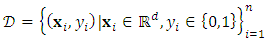(1)

Where d is the dimensionality of the feature vector and n is the number of instances in the dataset. In supervised learning the task is to find a generalized description of the class variable given a feature vector, that is, a classifier The classifier, optimizes some performance metric given the dataset,

2.2. Unsupervised Learning

In unsupervised learning, there are no class labels. An unsupervised learner rather seeks to cluster data that is similar. This paper does not emphasis unsupervised learning, but it is an essential preprocessing step used to understand data before putting it through a supervised learner. In an industrial setting, some data points are bound to be nonsensical, so called outliers. By making a supervised learner consider too many outliers will force it to not only model a complex non-linear system, but also model to the erratic behaviour of the outliers. Basically, a non-linear model is extrapolating across a discontinuity, which is not a sensible thing to do. Likewise, manufacturers might produce goods that are non-similar to each other. For example, a steel rolling mill might be rolling different alloys over time. Clustering data as preprocessing can greatly aid in the understanding of different production states, and different models based on supervised learning can be employed for the different clusters of data.

2.3. Overfitting and Validation

Machine learning models have a tendency to overfit with regards to the training data. Overfitting means that classifier has encoded noise within training data instead of finding the generalizing patterns in the dataset. To combat overfitting one usually samples the original dataset into subsets, i.e. training and validation sets. A training set is the one which the algorithm uses in order to approximate the class variable. The validation set is disjunct from the training set and is used to evaluate performance of a learner on unseen data. The trick is here to find the appropriate model complexity such that the learners performance on the validation set is maximized.

A popular way of assessing a models performance is to use k-fold cross-validation. The idea is to sample the dataset, into k equally sized disjunct subsets, For each fold, one of the subsets is held out as a validation set, while training the learner using remaining datasets, The performance is then measured as the mean performance for each fold. The strength of cross-validation is that the entire dataset will be used for both training and validation, where each point is validated exactly exactly once. Common practice is to perform 10-fold cross-validation to find appropriate model complexity.

3. Classifiers

This section will discuss some top performing classification algorithms. A brief presentation of the structure for each algorithm is provided. Discussion on training time, linearity, optimizing performance metric, and general performance for each algorithm is also provided.

3.1. Multilayer Perceptron

The multilayer perceptron (MLP) trained with backpropagation is arguably the most used and famous machine learning algorithm. Its usefulness has been proven in many industrial applications [8]. The MLP is a feedforward artificial neural network, and is simply a directed graph consisting of multiple layers of nodes. The most common structure of the network consists of three layers. One input layer, one hidden layer, and one output layer. More hidden layers can be used, but Cybenko [9] proved that a single hidden layer is sufficient to fulfil the universal approximation theorem.

Classification with an MLP containing one hidden layer with k hidden nodes is defined by two weight matrices, WandV, an activation function which operates element wise, and the Heaviside step-function, In this case, and The classification itself is expressed using Equation 2.

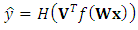(2)

The MPL is usually trained using backpropagation which is a gradient decent algorithm. As the name implies the gradient of prediction error is traced back through the network in order to appropriately update the weight matrices. Backpropagation can be performed both in batch and in an on-line manner. Wilson and Martinez [10] argues that the on-line variant is faster since a higher learning rate can be used without becoming unstable. When using backpropagation one should be aware that the produced MLP is deterministically dependent on the initial weights in W and V. These weights are usually initialized as near-zero white noise. Different local minima can be reached depending on these initial weights. Several networks with different initial values should be trained to ensure that the network does not get stuck in a poor performing local minima. However, LeCun argues that this is not necessary an issue in most real-world problems [11]. One property of backpropagation is that it minimizes Means Squared Error [12]. The MLP, therefore, performs well when evaluating a probabilistic performance metric, which is discussed in Section 5.3.

Training of MLP is slow compared to the other methods presented in this article. This is due to a large number or parameters which needs to be tuned. Some of the parameters to tune are: number of hidden nodes, weight decay, momentum, and learning rate. Grid search is the conventional approach for parameter tuning, but Bergstra et al. [13] argued that random search is more efficient, especially when the number of parameters to tune is large. Because of the slow training of the MLP, it is not particularity good at handling datasets with high dimensionality, especially when working with thousands of features. In this case, feature selection should be performed in order to achieve efficient training of the MLP, this is discussed in Section 7. According to Sharpe and Solly, backpropagation is poor at handling missing data and they proposed techniques to tackle this issue[14].

Many heavy industrial problems are basically descriptions of physical systems that are continuous in nature. In a certain vector space, MLP produces a linear discrimination boundary between classes which makes it naturally apt to work well on continuous problems.

3.2. Support Vector Machine

The foundations for Support Vector Machines (SVM) were laid in 1963 by Lerner and Vapnik [15]. The idea behind an SVM is to create a hyperplane that is as flat as possible and divides the feature space into two disjunct parts. The hyperplane divides the vector space such that there is a maximum margin between the two classes. The hyperplane defines a class boundary allowing new features to be evaluated to perform classification. A sample located under the plane is said to belong to one class, and vice versa. The initial idea was later extended to perform an implicit mapping into an infinite dimensional vector space via the so called kernel trick [16]. This enabled the SVM to perform classification on non-linear problems. Further improvements with soft margins were proposed in 1995 [17] allowing the SVM to work with dataset that were not separable by associating a cost to misclassification rather than forbidding it. Soft margins allow the SVM to work with noisy and mislabelled data. Since then the algorithm itself has remained relatively unchanged. The hyperplane itself can be expressed via a normal vector W and a bias b. Several researchers have found that the SVM is not the best performing general algorithm for classification [3] [5]. Nevertheless, it remains competitive due to its simple form. The SVM can be implemented on low grade hardware and the models are small in size and fast to evaluate.

When training an SVM, a quadratic programming problem is solved; there are readily available methods for solving these kinds of problems and training is relatively fast. SVM has a good ability to handle high dimensional data and is among the fastest algorithms for working with large datasets. As with MLP it is not natively adapted to handle missing and categorical data and encoding schemes are needed to enable this type of data. The SVM generally performs well on rank and threshold metrics in its basic form [18]. It is, however, not well suited for probability metrics, such as MSE, without calibration.

Due to the space transformation via the kernel trick, it is not trivial to analyse an SVM with regards to variable importance or inner workings of the model. This is the case when the classification problem is complex and high dimensional interactions are hidden in obscurity. Some indications of variable importance can be seen on the size of elements in the normal vector, W, that defines the hyperplane.

3.3. Decision Trees

One of the major strengths of the Decision Tree, DT, is that it is human interpretable. It is easy for domain experts, without knowledge in machine learning, to understand and analyse. The structure of the classifier itself is extremely simple, see Figure 1.

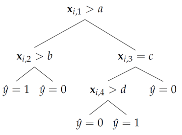Figure 1. The structure of a Decision Tree, where is estimated via logical tests of the features in a feature vector and are numerical or categorical constants determined by the learning algorithm

The DT is a binary tree which divides the feature space into hyper-rectangles at each node via a logical test. One leaf of the tree represents a hyper-rectangles via the boundaries defined by its ancestor nodes. Each leaf is assigned the class which best represents the training data that are located in its hyper-rectangle. The DT is fast to train and evaluate. Training is done using a top-down construction, with splitting criterion such as Gini impurity or information gain. The top-down construction is then followed by a bottom-up pruning process to remove leafs that lead to overfitting. The most popular DT algorithms are CART, C4.5, and C5.0. All of these algorithms share the same structure, but use different splitting criteria and pruning strategies in the tree construction.

The DT in its basic form is not considered a strong classifier but can be enhanced with bagging or boosting to achieve state-of-the-art performance, see Section 4. Unfortunately boosting or bagging will reduce the comprehensibility of the tree and increase the total size of the model. This makes them impractical to implement if target systems are restricted by storage constraints.

It is well known that DTs are good at maximizing threshold metrics, such as accuracy (ACC). Depending on how they are constructed they can also optimize rank metrics such as area under the curve[19]. The same article concluded that the DT is not well suited for probability metrics. Calibration techniques can be employed to remedy this.

3.4. Random Forest

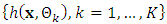
It is well known that it is possible to combine the predictive capabilities of multiple learners. This is something that the Random Forest (RF) exploits in order to produce a strong learner out of multiple weak learners. RF is an ensemble technique which combines multiple weak tree classifiers in a bagging procedure, see Section 4.1. The RF was introduced by Breiman [20] and is defined as follows:

"A random forest is a classifier consisting of a collection of tree-structured classifiers where the are independent identically distributed random vectors and each tree casts a unit vote for the most popular class at inputx."

What governs the strength of the RF is that each tree in the forest only sees a small part of the problem and specialize by only considering a small portion of the features. The individual trees in the forest are grown using the CART algorithm. Instead of letting the tree use all features, one samples p features which the tree is allowed to use as a basis for classification. Individual trees in the RF are not pruned, since bagging is used in the final prediction. It does not matter if individual trees overfit as long as there are sufficiently many trees in the forest as a whole. Breiman pointed to the strong law of large number to show that overfitting is not an issue for RF. It has also been shown that RF is robust against mislabelled, noisy, missing samples, and no special encoding scheme is needed. The RF is also fast in training, evaluation, and scales well with both training samples as well as high dimensional feature vectors. Few parameters need to be tuned making it easy to implement without much training and testing.

However, the Random Forest has some weaknesses that are apparent in industrial applications. Since RF is an ensemble algorithm, it produces a rather complex and hard to comprehend model. Looking at individual tree gives little insight regarding the full model and there is no clear way of visualizing the forest in its entirety. Furthermore, the model itself tends to be rather large which can prove a limitation for implementation on weak hardware.

Unlike learners such as SVM and MLP, neither of the tree learners produces a smooth surface in any vector space. This behaviour comes from the fact that the trees do binary splits. This enables the tree learners to work nicely on problems that are discrete, such as market forecasting [21].

4. Meta-Algorithms

In the search for stronger classification algorithms, researchers have devised methods for combining sets of classifiers to produce a single stronger classifier. These types of indirect strategies are called meta-algorithms with the most popular ones being Bagging and Boosting. These meta-algorithms can be used with any learner as they are generic methods. However, both Bagging and Boosting are commonly used only with DT or Stumps (DT having only a root node). As both Bagging and Boosting requires construction and assembly of multiple models, it is preferred to use with cheap modelling schemes.

4.1. Bagging

Bootstrap aggregation, or bagging for short, is an ensemble technique aimed at reducing variance and overfitting of a classifier. With regards to model performance, it never hurts to implement bagging. However, the drawback is that an ensemble of classifiers must be produced. As there are more models, there is a negative impact on training time, model size, and model comprehensibility.

Breiman [22] introduced the idea of bagging. Given a training set with size n, re-sample uniformly with replacements into m new datasets each with size Usually one chooses In this case, of the samples are expected to be unique within each of the produced subsets. The value of m should be sufficiently large in order to utilize all samples at least once. After re-sampling, a model of choice is fitted for each The final prediction is made by having a majority vote with all produced models, each being equally weighted.

Bagging is especially suitable when there are many features compared to the number of samples. For example, the number of changeovers for a manufacturer might be in the range of hundreds per year while the number of features are in the range of thousands. Bagging is also widely used in other fields where the number of features is large compared to the number of samples, such as bioinformatics [23].

Some learners, like RF, have bagging incorporated as a part of the algorithm itself and contributes to its strength in generalization. For these types of learners, there is no need to have extra bagging as post-improvement method of the produced classifier.

4.2. Boosting

Boosting is another meta-algorithm that is somewhat akin to bagging. However, instead of lowering variance it reduces the bias. Schapire [24] was the first to show that it was possible to construct a strong learner by combining a set of weak learners each of which just needs to perform better than random guesses. With boosting, it is possible to construct a classifier with arbitrary good classification ability with respect to the training data.

The most widely used boosting algorithm is AdaBoost constructed by Freund and Schapire [25]. The main idea of AdaBoost is to iteratively train weak classifiers and increase weights on training data which previous weak classifiers where unable to classify correctly. This procedure forces new learners to specialize and put more emphasis on previously misclassified samples. The weak classifiers are then weighted with regards to their general performance and the final output consist of a weighted vote. One of the biggest criticisms of boosting is that it is somewhat sensitive to faulty labelled training data. This is a problem since the boosting will tend to increase its efforts to classify the mislabelled data [26]. This leads to making boosting ill-suited for noisy data in real-world problems.

Boosting is a margin optimizing method and thus shares some properties with the SVM. Boosting models yields good performance in threshold and rank metrics but does not necessarily improve the probability metrics of the classifier.

5. Performance Metrics

Before choosing modelling algorithm, one should consider what type of classification problem that is to be solved and what exactly is to be optimized. There are three main types of metrics which are often interesting in classification and different algorithms are apt to optimize different performance metrics. Three common families of performance metrics are investigated.

1. Threshold Metrics: Classifiers often produce an output between 0 and 1. This output does not necessarily reflect the probabilities of the output belonging to one class or the other. A threshold metric defines a discrimination threshold, usually 0.5, which is used to discriminate output to the two classes. A threshold metric measures the rate of correctly classified examples given athreshold. Examples of threshold metrics are ACC and F₁-score. A Threshold Metric is suitable if one needs a classifier that is correct in a certain rate of the cases. Class distribution greatly affects threshold metrics performance and the class distribution should be comparable between training data and operational data when threshold metrics are used.

2. Rank Metrics: A rank metric measures how well a classifier is able to rank outputs with regards to the class. The actual predicted values are not interesting for the rank metrics but rather how well the output values reflects the ordering of the two classes. AUC is arguably the most commonly used rank metric and will be described later in this section.

3. Probability Metrics: A probability metric gives a measure of the expected probability of a learner’s output to be correctly classified. Well calibrated models, such as MLP, are designed such that they minimize a probability metric. This means that one can judge how probable an output is to be correctly classified. In an industrial setting one can, for example, estimate the probability of achieving desired output given certain actions. Mean squared error (MSE) belongs to the class of probability metrics. Probability metrics has gained the reputation to be good at assessing the general performance of a learner. This is so since a learner that performs well on a probability metric naturally performs well on a rank metric but not necessarily the other way around [19].

5.1. Accuracy

ACC is a metric to assess proportion of true results among the total number of samples evaluated in binary classification problems. It ranges between 0 and 1, where 0 means no examples were correctly classified and 1 means that all examples were correctly classified. A binary classifier can achieve four results given a validation set:

● TP: True Positives, the number of examples in the positive dataset which are correctly classified.

● TN: True Negatives, the number of examples in the negative dataset which are correctly classified.

● FP: False Positives, the number of examples in the positive dataset which are incorrectly classified (classified as the negative dataset).

● FN: False Negatives, the number of examples in the negative dataset which are incorrectly classified (classified as the positive dataset).

ACC in its standard form is calculated using Equation 3.

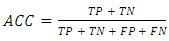(3)

ACC is a threshold metric and only consider a single threshold, usually 0.5. This means that ACC can be misleading if the learner is trained on imbalanced classes. The learner can, in such cases achieve high accuracy without having any sensitivity whatsoever. By associating weights to FN and FP the impact of different types of errors can be adjusted in accordance to its severity. Classifiers produces an output and a discrimination threshold is used to determine if the output should belong to one class or the other.

5.2. Area under Curve

The Receiver operating characteristic curve (ROC) considers False Positive Rates (FPR) and True Positive Rates (TPR) at different thresholds. FPR and TPR are calculated with to Equation 4.

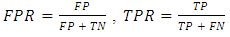(4)

If one plots the FPR against TPR for all discrimination thresholds, ROC-curve is obtained. The ROC is rich in information regarding the performance of the classifier at different thresholds but since it is a graph it needs to be converted into a scalar in order to be considered as a proper performance metric. One can integrate the ROC to get the area under the curve (AUC). The AUC describes the probability that a classifier given a randomly chosen positive example ranks it over randomly chosen negative one and is, therefore, called a rank metric [27].

5.3. Mean Square Error

Mean Square Error (MSE) is a metric which incorporates both the bias and variance of the predictor which has made it into one of the most popular performance metrics for classifiers. MSE of an classifier, is calculated as follows:

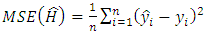(5)

It also expresses the expected squared error of the estimator, where H is the true classifier. With the standard definition of variance, the MSE can be reformulated as:

(6)

It is the combination of these statistical entities that makes MSE such a popular performance metric. The MSE thus provides insights in both how biased an classifier is as well as how precise a classifier is.

5.4. Combined Metric

In many cases, it is not possible to know what performance metric to use for the classifier in order to best emulate a certain problem. Caruana et al. [28] performed an extensive analysis of different performance metrics and their correlations for a wide set of problems. The authors formed a novel metric called SAR which combines ACC, AUC and MSE, as described in Equation 7.

(7)

They claimed that this to be a robust metric when the correct metric is unknown. One can compare different families of classifiers against each other using this fair metric.

6. Calibration

Some machine learning methods such as SVM and DT are notoriously bad at optimizing probability metrics of the classification outputs. A way of addressing the poor probability estimation from models is to introduce calibration. Calibration maps a model’s output in an injective monotonic manner. This means that rank metrics are unaffected by calibration while improving the probability metrics. Models that have the most to gain from calibration are the margin maximizing ones, such as SVMs and boosted models. In this section two calibration techniques, Platt scaling and Isotonic regression, are discussed. At the end of the section some conclusions are presented.

6.1. Platt Scaling

Platt scaling [29] is a post-training calibration method to address the issue of poor probability estimations. The method was originally designed to work with SVMs, but has proven useful for other learning algorithms as well. Platt scaling estimates the probability of an output belonging to the positive class given a feature vectorx. That is, Platt argued from empirical experience that a logistic regression, as illustrated in Equation 8, is a good transformation of outputs for many real world problems.

(8)

Where the parameters A and Bare estimated using maximum likelihood methods described by Platt. The author showed that the post-calibration with SVM and sigmoid yielded probabilities of comparable quality to regularized likelihood methods.

6.2. Isotonic Regression

Isotonic regression is another calibration method. It has been shown to supersede the Platt scaling in problems regarding multi-class probabilities, the Isotonic regression also provides better computational scaling with regards to the number of samples [30].

In contrast to Platt scaling, which is parametric method, the Isotonic regression only assumes that probabilities are monotonically increasing or decreasing. This is a more general assumption. Meaning that Isotonic regression is better suited for a wider range of problems where the output distribution is not limited to logistic-curves.

Isotonic regression performs a weighted least-square approximation, in which the PAVA-algorithm [31] is used to solve the QP-problem in Equation 9. The PAVA-algorithm itself operates in linear time, O(n), and sweeps through the data and re-adjusts the estimator’s output for the points which violates the monotonicity constraint.

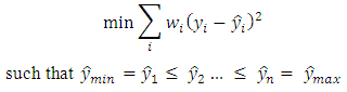(9)

6.3. Choosing Calibration Technique

As another training set is needed for the calibration, Platt calibration is preferred when there are only a few training examples to spare for calibration. This is because it uses maximum likelihood estimates. If there is an abundance of post-calibration samples, Isotonic regression is preferred due to its fast execution.

Methods that are naturally well-calibrated, such as MLP or bagged trees, get little to no benefit and sometimes even worse performance after calibration. If these methods are to be implemented calibration is not needed [32].

When choosing between Platt scaling and Isotonic regression, Figure 2 can be consolidated in order to select between the two calibration strategies.

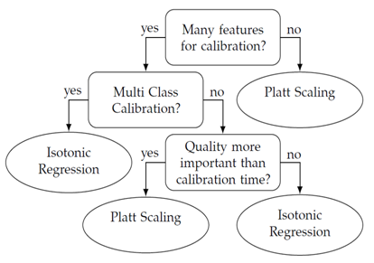Figure 2. Decision process to chosecalibration technique

7. Feature Selection

Given a dataset, consisting of N samples and M features The task of the feature selection is to find a compact subset 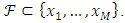Where imposes no significant loss in predictive information regarding the target class compared to

When working with thousands of different features, some are bound to be important in describing the process while others are virtually meaningless. There are three main objectives in feature selection:

1. Provide better insight in the underlying process. If the dimensionality of the problem can be reduced, it becomes easier for domain experts to analyse and validate produced models.

2. Since machine learning algorithms fits their view of reality based on the data, they is trained on they can have a tendency to find patterns within noise. Meaning that if there are too few samples with a high dimensionality, there is a substantial risk that a model encodes the noise and overfits. With a compact feature set better generalization can be achieved.

3. If a predictor is to be implemented limitation of the feature set makes models both smaller, faster and more cost-efficient.

When choosing feature selection approach there are, as always, multiple things to consider. Things regarding optimality of feature sets, time taken to perform feature selection, complexity of the problem to model, and the actual structure of the data. For more discussion regarding the subject see Guyon and Elisseeff’s introduction to feature selection [33].

In feature selection, there are three main classes of methods for performing the selection of variables, namely wrappers, filters, and embedded methods.

7.1. Wrappers

Wrappers iteratively creates subsets of features which are used to form models. These models are trained and validated on a hold-out validation set. This is done in order to measure the error rate given different feature-subsets. The advantage of wrappers is that they can be tuned and evaluated on specific modeling algorithms. Wrapper methods have the ability to find best feature set, but wrappers are unfortunately computationally expensive since there are combinatorially many feature sets to train and evaluate. The combinatorial possibilities in feature sets often makes a wrapper infeasible to use on large scale problems. If the feature set is large, some search strategy is needed, such as best-first, branch-and-bound, simulated annealing or genetic algorithms [33].

7.2. Filters

Due to the computational costs of wrappers, filters have gained support in many real-world applications. Filter methods do not consider what model is to be implemented in the end. They analyse rather correlation between feature variables and the class variable. Two popular filter techniques are Correlation-based Feature Selection (CFS) [34] and Fast Correlation-Based Filter (FCBF) [35] were both share the same heuristic for selecting features:

“A good feature subset is one that contains features highly correlated with (predictive of) the class, yet uncorrelated with (not predictive of) each other.”

Both CFS and FCBF consider two-way interactions between the features which means that they are able to find features that are closely correlated with the class. More complex feature interactions are, however, not detected and filtered out. Filter techniques generally culls the feature set hard and only detects the top-most important features. Giving the ability to find feature sets that are good for generalization often leads to slight loss in predictive capability if complex feature interactions occur.

7.3. Embedded Methods

Embedded methods have emerged as a middle ground between the filter and wrapper methods. An embedded method incorporates a natural machine learning technique in its feature selection. This avoids the combinatorial explosion seen in the wrapper methods, while not just looking at correlations as in a filter method. There is a number of different embedded methods which have gained popularity. Two of the most popular ones are SVM with recursive feature elimination (SVM-RFE) and Regularized Trees.

SVM-RFE works by training an SVM with the entire feature set. At each iteration, the feature with the lowest weight in the W-vector is removed and performance stored. At the end, a performance profile can be plotted and one can chose the smallest feature set with the best performance. Other learners than SVM can be used for RFE but due to SVMs great ability of working with high dimensional data, it is often preferred.

Regularized Trees (RT) proposed by Deng et al. [36] is an computational efficient technique based on ensemble tree learners. As with other tree learners, it can handle categorical and continuous data naturally. The idea behind RT is to penalize the use of the same feature in multiple nodes. This strategy forces the RT to consider a wider range of features in the building of the trees. RT generally selects a larger set of features compared to the filter techniques.

At the same feature set size, both algorithms achieve comparable performance. However, as the SVM-RFE must train one classifier per size of the feature set, it takes more computational effort to reach the same feature set size compared to RT. However, with the performance profile of the SVM-RFE, one can on the other hand chose the number of features desired to use.

8. Classification in Continuous Manufacturing

In this section, techniques previously discussed in this article together with some practical examples of how they have been utilized in real world problems are presented.

8.1. Feature Selection

A field very different albeit similar to heavy industrial manufacturing is Bioinformatics and genetics. These fields face a similar problem with feature selection, as there are usually a high number of features compared to samples. In both areas, feature selection is essential to gain knowledge regarding the underlying mechanics of the system to be analysed.

Deng et.al [37] compared Regularized Random Forests with the more conventional feature selection technique LASSO [38]. In total 10 genetic classification problems were evaluated. None of these problems had more than 102 samples and none had less than 2000 features. When the sample/feature ratio is this low, feature selection is essential for gaining knowledge within the data. The authors found that the regularized random forest feature selectors generally produced a larger feature sets which captured more of information regarding the class variables. For a strong classifier such as RF, this is a clear advantage while a weaker DT will not benefit from the larger feature set since it unable to capture the complex feature interactions anyway. The authors also discussed the convenience of not needing to pre-process the data with RRF.

8.2. MLP Examples

MLP was the first algorithm which really takes off in an industrial setting and has seen many uses since its popularity began to rise in the early 1990’s. Meireles et al. [8] performed a comprehensive review of industrial applications using MLPs. There is no shortage of applications in continuous manufacturing where MLPs has been employed in the real world. Kandroodi et al. [39] used an MLP to identify the dynamical behaviour of continuously stirring tank. Further, the neural network was also used for predictive control of the system. Singh et al. [40] used MPLs to model and control a non-linear continuous chemical process. Weng et al. [41] used bagged MLPs to successfully predict curl of paper in paper manufacturing.

As discussed earlier, MLP generally are quite expensive to train and are unable to handle missing and categorical data. Preprocessing is essential but when correctly tuned the MLP is an excellent model for a wide range of problems.

8.3. SVM Examples

Due to its good generalization and ability to produce a smooth classifier, SVM has been a popular tool in industrial applications. In a survey by Saybani et al. [42] the uses of SVM within oil refineries where examined. Some of the uses were classification of gasoline, classification of gases, and prediction of electrical energy consumption.

In an article by Xu el.al [43] an MPL and SVM were compared. Both learners were used to predict yield from a furnace used in steel production. As remarked earlier both MLP and SVM produces a hyperplane which discriminates the classes. The authors states that the models can be transformed into each other. However, the SVM has a better ability to make a trade-off between model complexity and predication precision. Moreover, the SVM is better at avoiding over-fitting which makes it especially interesting when there are few training examples.

In paper production, the so called Kappa number is an interesting quality measure of the paper pulp. Measuring this quality directly with on-line sensors is hard. Li et al. [44] proposed SVMs as a means of inferring the Kappa number from measurements of surrounding sensors. In this experiment the SVM outperformed an MLP.

8.4. Decision Tree Examples

As mentioned earlier, the DT rarely achieves top performance in its basic form. It has, however, seen uses due to its human interpretability. For example, in a report by Coopersmith et al. [45], the authors discusses the usage of Decision Trees in oil and gas industry. They concluded that DT to be useful tools to get an hierarchical overview of variable importance as an aid in decision making. They specifically presented examples where a company should decide if it is worth drilling on a test sight or not.

Aghdam et al. [46] found that single decision trees were unable to produce sufficiently good fault detection accuracy compared to MLP and SVM in a steel production facility. The authors suggested and implemented bagged decision trees which were able to outperform the conventional DT, MLP and SVM.

For stronger classification, bagging or boosting should be employed. For example, Halawani [47] used decision trees in combination with AdaBoost to perform fault detection of steel plates with good accuracy.

8.5. Random Forest Examples

RF is yet to be widely employed in industrial applications but has proven to be useful in a number or areas that involves modeling of complex continuous systems such as electricity markets [21] or prediction of transitions between weather regimes [48].

Berrado et al. [49] modeled Thixoforming in a steel making process in order to find operational parameters and how they affects the quality of the produced good. The authors used a RF to model this process and determined appropriate operational conditions to improve the forming load.

Further, Laha et al. [50] used RF to model the yield of an open hearth steel manufacturing process. In this study, several learning algorithms such as SVM and MLP are discussed and used for the same problem. The authors found that SVM worked best for this particular problem.

Auret et al. [51] performed an analysis of how RF could be used within mineral processing, which is a continuous process that is highly complex and hard to analyse with linear models. The authors found the RF to be a practical tool for root cause detection of abnormal behaviours. The RF were able to handle highly non-linear relationships between features and class variables. Comparing with other classifiers such as MLP and DT, the RF are able to perform analysis of complex feature interactions. However, the authors pointed out that RF models might be impractical to implement into existing systems but can act as strong analytical tools for extracting knowledge from historical data. The authors pointed to a big advantage with RF in that users need not be overly concerned with tuning of parameters or other issues related to model specification. The algorithm’s strength in handling missing and noisy data is another advantage.

Kotsiantis et al. [52] used a RF to estimate tissue softness in paper production. This is an important quality measure. The authors found that the RF outperformed other learners in this problem.

9. Future Work

This article will serve as a guideline for implementation of a classifier in one of Sweden’s largest paper mill. When changing the type of paper that is produced the paper pulp must be treated in advance to fulfil certain requirements. More specifically, a bleaching process of the paper pulp needs to be initiated hours before being used. The time it takes to bleach paper pulp is hard to predict since the process is affected by multiple variables that interact non-linearly. These variables are non-trivial to incorporate into a classical modelling scheme as they are both categorical and numerical as well as noisy or missing.

First on the agenda is to evaluate the accuracy of the current bleach time model. The paper mill has recorded performance and set variables for years and this data will be used to analyse the historic predictive performance of the current model.

It is known that the current model is largely simplified and only accounts for a small number of parameters that actually determines the bleach time. The different feature selection techniques discussed in this article will be employed in order to identify relevant variables as well as reducing the size of the massive feature set to enable modelling based on machine learning techniques. Domain experts at the paper mill will aid in the validation of the selected feature set.

Finally, models described in this article will be implemented to see if they can outperform the current solution with regards to increased accuracy of the bleach time prediction. With access to large amounts of historical data there is good potential that an improved model can significantly reduce the expected change overtime.

10. Summary

As seen throughout this entire article there are many ifs and buts when choosing a modelling scheme. In this section loose ends are tied together and future directions are provided. With the reservation that there are exceptions that contradicts these rules!

10.1. Selecting Features

Given cleaned data that is clustered it in such a way that each individual cluster of data is consistent and ready to be modelled. The first decision faced is that of feature selection. Does it make sense to reduce the dimensionality of the data set? In an industrial context, with possibly thousands of features, feature selection most often makes sense! Not all setpoints and sensor readings can possibly be useful descriptors for the classification. The feature selection might also be one of the most important tools for domain experts to validate and gain insight in the produced models. With a more compact feature set it is easier to appreciate and visualize the characteristics of the data. Figure 3 shows a simplified decision tree which summarizes Section 7. Consolidate this figure when choosing feature selection technique. It is worth noting that wrappers is an attractive approach if there are sufficient computational resources available to perform the feature selection, although smart search techniques need to be employed even if the problem is relatively small.

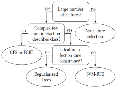Figure 3. Decision process for whatfeature selection technique to employ

10.2. Selecting Type of Metric

At this point it is time to decide what performance metric the machine learner is going to optimize against. In the list below situations are described that should be considered.

● The class distribution in the training data corresponds well with future operational data and the classifier should be able to make the correct classification in a certain percent of the cases. Then chose threshold metric.

● The most important thing is to get good ordering between positive and negative examples. That is, given one random positive example and one random negative one, and the goal is to to maximize the chance of ranking the positive examples above the negative class. Then chose rank metric.

● If good ranking ability is sought as well as the ability to perform statistical analysis of the efficiency of the predictor a probability metric is suitable. As it allows individual example to be analysed with regards to the certainty of the prediction.

Probability metric generally contains the most information regarding a classifiers strength and is therefore often a preferred metric. Unless a well calibrated learner is used, such as MLP or Bagged DTs, post-calibration is needed in order to yield good probability metrics. Consolidate Figure 2 in Section 6 if choosing between Platt scaling or Isotonic regression.

10.3. Selecting Model

10.3.1. Best in Class

If computational resources is not a limiting factor the ensemble techniques generally tends to perform the best. These techniques are able to produce robust models with high accuracy. Also no special attention needs to be put to data normalization or missing values. They handle high dimensions well and natively performs variable ranking which can be measured. The models themselves are, however, quite large and hard to interpret.

● On threshold metrics RF generally achieve uncontested performance.

● On rank metrics all three ensemble learners, BST-DT, BAG-DT and RF achieve good general performance.

● On probability metrics the calibrated BST-DT generally has best performance [3].

10.3.2. Bound by Reality

Many industrial facilities utilize old computer hardware. As the ensemble techniques tends to produce models that are big, they are not always feasible to implement directly into the existing hardware. In real world applications this can be a serious obstacle which hinders implementation of these models into the production facility. In these cases a slightly weaker classifier might suffice.

● MLP generally performs well under all performance metrics but are, unfortunately, expensive to train. They can produce compact models consisting of only two matrices. Evaluation is fast and they do not need probabilistic calibration.

● SVM is terrible with regards to probability metrics, and require calibration in order to handle such metrics. That said they can produce a compact classifier with good generalization abilities over the entire feature space.

These two classifiers produces continuous hyperplanes, which enables them to make classification over the entire feature space. Whereas the tree based learners cannot extrapolate outside the bounds of the training data.

The DT rarely produces competitive classification performance. It is, however, easy to interpret and can be useful tools for educational purposes. It can be used to produce a simple rule based decision support tool which can be printed on a paper and used by humans.

11. Conclusions

Selecting a strategy for binary classification in an heavy industrial setting is no trivial task. There are many things to consider and aspects to take into consideration as discussed in this article.

Firstly the use of feature selection is encouraged, especially in heavy process manufacturing where the number of features are often in the range of thousands. There is a clear need to structure and understand data in order for domain experts to validate and analyse produced models.

Examples where classifiers are compared without considering what performance metric each algorithm are apt to optimize have been seen throughout literature. This article has summarized under which conditions different learning algorithms are expected have good performance. Further, the use of calibration techniques is encouraged since most learners naturally are uncalibrated with regards to probabilistic performance metrics.

Finally, examples from continuous process manufacturing where machine learning classifiers has been employed for different problems has been presented. Some general patterns under which circumstances different learners are appropriate has been observed and the article has commented on these characteristics. Both from a practical industrial point of view as well as some theoretical limitations of the different learners.

A general conclusion is that ensemble learners based on trees often produces the strongest classifiers in an industrial setting due to their excellent generalization ability as well as their natural ability to handle missing and noisy data.

As a second best alternative SVM possess many nice properties in that they handle high dimensional data well, produce a compact model and give some insight into variable importance.