-
Paper Information
- Paper Submission
-
Journal Information
- About This Journal
- Editorial Board
- Current Issue
- Archive
- Author Guidelines
- Contact Us
American Journal of Intelligent Systems
p-ISSN: 2165-8978 e-ISSN: 2165-8994
2015; 5(2): 64-72
doi:10.5923/j.ajis.20150502.03
Self Organized Grouping of Ears Based on Inertia Related Biometrics Using Kohonen’s Feature Map
 Abstract
 Reference
 Full-Text PDF
 Full-text HTML
Prashanth G. K., M. A. Jayaram, Gaddi Siddharam
Department of MCA, Siddaganga Institute of Technology, Tumkur, Karnataka, India
Correspondence to: Prashanth G. K., Department of MCA, Siddaganga Institute of Technology, Tumkur, Karnataka, India.
| Email: |  |
Copyright © 2015 Scientific & Academic Publishing. All Rights Reserved.
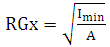
Classification of images based on the biometric features is a challenging problem in the field of pattern recognition and person identification. In this paper, we propose a Self Organized Feature Map (SOFM) to group ears for the purpose of person identification. A database of 605 right ear images is used to develop the recognition system. The application of SOFM permitted to differentiate four classes of ears. The features used are novel and are based on the Moment of Inertia (MI) related parameters. To elicit the parameters the ear is considered to be planner surface. Five parameters namely MI with respect to major axis and minor axis, radii of gyration (RG) with respect to major axis and minor axis, and the planner area of the ear were considered. The results show that four groups are distinct with minimum overlapping. The group characteristic has also been reported. The significance of this work is seen in decreased grouping and image retrieval time to an extent of 10% when the images in the database is organized in blocks of groups when compared to image matching and retrieval time when unorganized database is considered.
Keywords: Ear biometrics, SOFM, Moment of inertia, Radii of gyration, Major axis, Minor axis
Cite this paper: Prashanth G. K., M. A. Jayaram, Gaddi Siddharam, Self Organized Grouping of Ears Based on Inertia Related Biometrics Using Kohonen’s Feature Map, American Journal of Intelligent Systems, Vol. 5 No. 2, 2015, pp. 64-72. doi: 10.5923/j.ajis.20150502.03.
Article Outline
1. Introduction
- Biometrics is basically identification or self verification by taking personality information that corresponds to an individual [1, 2]. Biometrics can be categorized into two types, which are behavioural and physical [3].The human ear is becoming a popular biometric feature in recent years. It has several advantages over other biometric technologies such as iris, fingerprints, face and retinal scans. Ear is large when compared with iris and fingerprint. Further the image acquisition of human ear is very easy as it can be captured from a distance without the cooperation of an individual [6]. Human ear contains rich and stable features and it is more reliable than face as the structure of ear is not subject to change with the age and facial expressions. It has been found that no two ears are exactly the same even that of identical twins [7, 8]. Therefore, it is proved beyond doubt that the ear biometrics is a good solution for computerized human identification and verification systems. The major application of this technology is in crime investigation. Ear features have been used for many years in the forensic sciences for recognition.A profound work of ear identification involving over 10000, ears has been documented [4]. In an experiment involving larger datasets more rigorously controlled for relative quality of face and ear, the recognition performance was almost same when ear and face were individually considered. However, the performance shot up to 90.9% when both ear and face were considered [3]. Ear biometrics is an unexplored biometric field, but has received a growing amount of attention over the past few years. There are three modes of ear biometrics: ear photographs, ear prints obtained by pressing the ear against a flat plane, and thermograph pictures of the ear. The most common implementation of ear biometrics is via photographs for identification systems [4].The rest of the paper is organised as follows. Section 2 elaborates on related Works; Kohonen’s Feature Map is briefed in section 3. The way in which the data was acquired is explained in section 4. Moment of inertia (MI) based feature extraction is presented in section 5. The result and discussion are made in section 6, and the paper concludes in section 7.
2. Related Works
- Literature survey revealed a wide spread application of Artificial Neural Networks in biometrics. However the application of SOFM in biometric seems to be scare. Mai V et al [9] proposed a new method to identify people using Electrocardiogram (ECG). QRS complex (Q waves, R waves, S waves) which is a stable parameter against heart rate variability is used as a biometric feature. This work has reported for having achieved a classification accuracy of 97% using RBF.Sulong et al [10] have used a combination of maximum pressure exerted on the keyboard and the time latency between the keystrokes to recognize the authenticate users and to reject imposters. In this work, RBFNN is used as a pattern matching method. The system so developed has been evaluated using False Reject Rate (FRR) and False Accept Rate (FAR). The researchers have affirmed the effectiveness of the security system designed by them. Chatterjee et al [11] have proposed a new biometric system which is based on four types of temporal postural signals. The system employs S-transform to determine the characteristic features for each human posture. An RBFNN with these characteristic features as input is developed for specific authentication. The training of the network has augmented extended Kalman filtering (EKF). The overall authentication accuracy of the system is reported to be of the order of 95%.In a study, multi-modal biometric consisting of fingerprint images and finger vein patterns were used to identify the authorized users after determining the class of users by RBFNN as a classifier. The parameters of the RBFNN were optimized using BAT algorithm. The performance of RBFNN was found to be superior when compared with KNN, Naïve Bayesian and non-optimized RBFNN classifier [12].Ankit Chadha et al have used signature of persons for verification and authentication purpose. RBFNN was trained with sample images in the database. The network successfully identified the original images with the recognition accuracy of 80% for image sample size of 200 [13].Handwriting recognition with features such as aspect ratio, end points, junction, loop, and stroke direction were used for recognition of writers [14]. The system used over 500 text lines from 20 writers. RBFNN showed a recognition accuracy of 95.5% when compared to back propagation network.Enhanced Password Authentication through Typing Biometrics with the KMeans Clustering Algorithm. [16]. Combination of supervised and unsupervised learning for clustering data without any preliminary assumption on the cluster shape is implemented for Iris dataset [17]. A new method directed towards the automatic clustering of x-ray images. The clustering has been done based on multi-level feature of given x-ray images such as global level, local level and pixel level. [18].Suad K. Mohammad [19], have used a new method for Ear Recognition by Using Self Organizing Feature Map, They have developed and illustrated a recognition system for human ears using a Kohonen self-organizing map (SOM) or Self-Organizing Feature Map (SOFM) based retrieval system.
3. Kohonen’s Feature Maps
- The Self-Organising Map (SOFM) network performs unsupervised learning. It is neural network that forms clusters that reflect similarities in the input vector. It is mapping that defined implicitly and not explicitly. This is desirable because this investigation is not restricted to any particular application or predefined categories. Input vector vector are presented sequentially in time without specifying the output. Because of the fact, their is no way of predicting which neurons will be associated with a given class of input vectors. This mapping is accomplished after training the network. The SOFM has sequential structure starting with the d input vector (input neurons) x, which are received by the neurons in parallel and scaled by the weight vector w. Thus the weight matrixes the size of neurons by d inputs. The n neurons are then entered into competition where only one neuron wins. This architecture of the SOFM is illustrated in Fig.1. SOFM employs the concept of topological neighbourhoods, which are equidistance neuron neighbourhoods centred around a particular neuron. The neighbourhood centred around a particular neuron. The neighbourhood distance matrix for a one-dimensional case using four neurons is:
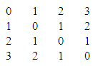 It can be seen that the distance of neuron from itself is 0, the distance of neuron from its immediate neighbour is 1, and so on.
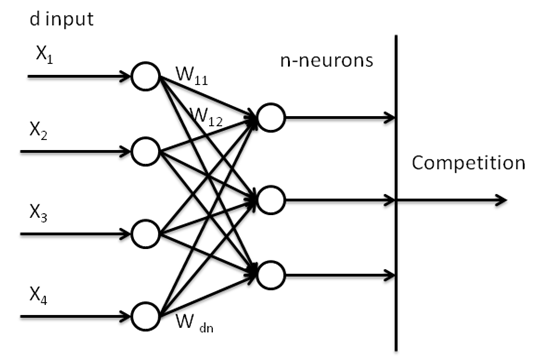 | Figure 1. Architecture of Kohonen Feature Map |
 | (1) |
 | (2) |
3.1. SOM Sample Hits
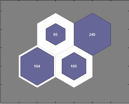
- SOM hits calculates the classes for each neuron and shows the number of neurons in each class. Areas of neurons with large numbers of hits indicate classes representing similar highly populated regions of the feature space. Whereas areas with few hits indicate sparsely populated regions of the feature space [20-24].The default topology of the SOM is hexagonal. This figure shows the neuron locations in the topology, and indicates how many of the training data are associated with each of the neurons (cluster centres). The topology is a 2-by-2 grid, so there are 4 neurons. The maximum number of hits associated with any neuron is 240 and minimum is 65. In this work, 5x605 matrix is considered as input data. After clustering using SOFM 605 data were divided in to 4 neurons (clusters). First neuron hit 194 times, second neuron hit by 105 times, third by 65 and forth by 240. Such sample and hits are shown in Figure 2.
 | Figure 2. SOM Sample Hits |
3.2. SOM Topology
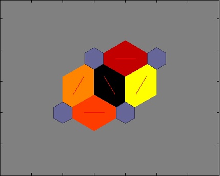
- SOM training, the weight vector associated with each neuron moves to become the centre of a cluster of input vectors. In addition, neurons that are adjacent to each other in the topology should also move close to each other in the input space, therefore it is possible to visualize a high-dimensional inputs space in the two dimensions of the network topology. The default SOM topology is hexagonal [25].
3.3. SOM Neighbour Connection
- SOM Neighbour Connection shows the SOM layer, with the neurons denoted as a dark patches and their connection with their direct neighbour denoted as line segment. Neighbour typically classify similar sample. [26]
3.4. SOM Neighbour Distance
- SOM Neighbour weights distance shows to what extent (in terms of Euclidian distance) each neuron classes are from its neighbour. Connections which are bright indicate highly connected areas of the input space. While dark connection indicates classes representing regions of the feature spaces which are far apart, with few or no neurons between them.
 | Figure 3. SOM Neighbour Distance |
3.5. SOM Input Planes
- SOM Plane shows a weight plane for each of the five input features. They are visualization of the weights that connected each input to each of the 4 neurons in the 4x4 hexagonal grid. Darker colour represents larger weights. If two inputs have similar weights planes (their colour gradients may be the same or in reverse) it indicates they are highly correlated.
4. Data Acquisition
- The ear biometric recognition systems can also be divided into five main parts - image acquisition, pre-processing, feature extraction, extraction of feature vector and classification & comparison [3]. The process of ear edge extraction is shown in Figure 4. A typical edge of the ear is also shown in Figure 5.
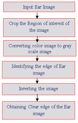 | Figure 4. The Steps involved in ear edge extraction |
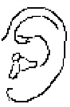 | Figure 5. The Outer Edge of Ear (Typical) |
5. Feature Extraction
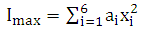
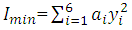
- To start with, the major axis and minor axis were identified. Major axis is the one which has the longest distance between two points on the edge of the ear, the distance here is the maximum among point to point Euclidean distance. The minor axis is drawn in such way that it passes through tragus and is orthogonal to the major axis. Therefore, with different orientation of ears the orientation of major axis also changes. Being perpendicular to major axis, the orientation of minor axis is fixed. The surface area of the ear is the projected area of the curved surface on a vertical plane. This area is assumed to be formed out of segments. Only the area of an ear to the right side of the major axis is considered to be made out of six segments. Each of the segments thus subtends 30° with respect to the point of the intersection of the major axis and minor axis. The extreme edge of a sector is assumed to be a circular arc. Thus converting each segment into a sector of a circle of varying area. One such typical segment is shown in figure and a measurement involved over such segment is presented in Figure 6.
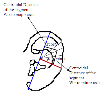 | Figure 6. Segments of Ear |
 | (1) |
 | (2) |
 | (3) |
 | (4) |
 | (5) |
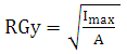
5.1. Shape Based Biometrics
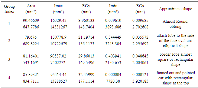
- The five shape based features of ears that were considered for classification are listed in the Table 1. The details of feature extraction and their evaluation authentication and validation are available in seminal work of authors [27]. However, for the sake of clarity, the features are briefly explained in the following paragraphs.
|
6. Result and Discussion
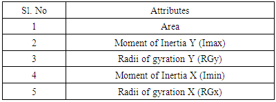
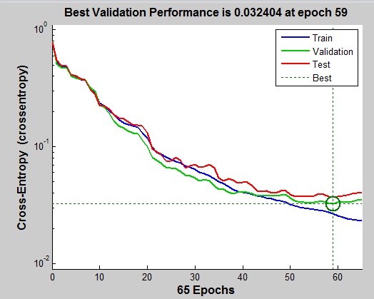
- Table 2 shows the sample database used for this work. From Figure 7, it is evident that the errors involved during validation are at lower level when compared to errors that happened during training. The histogram is indicative of the fact the low errors in the range of - 0.04318 and 0.04318 for most of the samples. The training errors are also to the tune of 0.0886 which is very low.
|

 | Figure 7. The Mean Square Error |
 | Figure 8. Error Histogram |
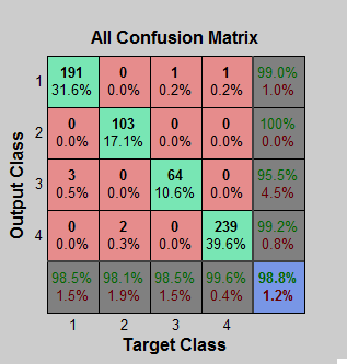 | Figure 9. Confusion Matrix |
|
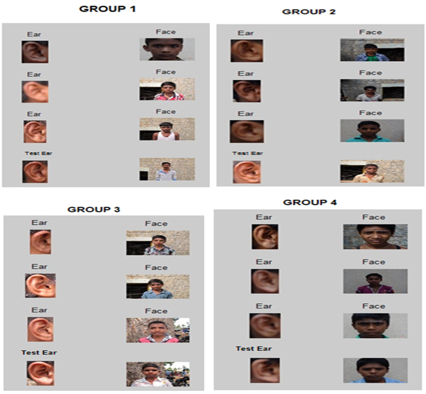 | Figure 10. Test images and a small segment of the corresponding Group |
7. Conclusions
- This paper presented SOFM based image matching and personal identification. SOFM provided four subset of ears with typical characteristic features. To effectively utilize SOFM generated groups the matching of test ear images was done on ear image database which was organised as per groups. This resulted in reduction of CPU time for matching and retrieval of images to an extent of 10% when compared with the time taken for matching and retrieval of the same in unorganised ear database.