Hasan Fleyeh, Barsam Payvar
Computer Engineering Department, School of Technology and Business Studies, Falun, Sweden
Correspondence to: Hasan Fleyeh, Computer Engineering Department, School of Technology and Business Studies, Falun, Sweden.
| Email: |  |
Copyright © 2015 Scientific & Academic Publishing. All Rights Reserved.
Abstract
This paper elaborates the routing of cable cycle through available routes in a building in order to link a set of devices, in a most reasonable way. Despite of the similarities to other NP-hard routing problems, the only goal is not only to minimize the cost (length of the cycle) but also to increase the reliability of the path (in case of a cable cut) which is assessed by a risk factor. Since there is often a trade-off between the risk and length factors, a criterion for ranking candidates and deciding the most reasonable solution is defined. A set of techniques is proposed to perform an efficient and exact search among candidates. A novel graph is introduced to reduce the search-space, and navigate the search toward feasible and desirable solutions. Moreover, admissible heuristic length estimation helps to early detection of partial cycles which lead to unreasonable solutions. The results show that the method provides solutions which are both technically and financially reasonable. Furthermore, it is proved that the proposed techniques are very efficient in reducing the computational time of the search to a reasonable amount.
Keywords:
Combinatorial Optimization, Cable Cycle Routing Problem, Reliability of Path, Conditional Directed Graph, Admissible Heuristic Estimation
Cite this paper: Hasan Fleyeh, Barsam Payvar, Optimization of Cable Cycles: A Trade-off between Reliability and Cost, American Journal of Intelligent Systems, Vol. 5 No. 2, 2015, pp. 43-57. doi: 10.5923/j.ajis.20150502.01.
1. Introduction
Cable routing problem, which this paper addresses, is a problem that arises when an organization installs a set of devices (called objects) in a building as well as ladders (called routes) to support the cables. The problem is how to direct a cable through the routes to link a subset of objects, such that the path forms a cycle (i.e., starting and ending at the same object) provided that it should be financially and technically feasible. The financial concern is the length of the cable path, while the technical concern is relevant to the reliability of the path in case of link failures. Since the organization has not clearly defined a measure for the reliability, the authors have elucidated an efficient measure in this work.Among the objects linked together by the same cable, there is a cabinet called the primary object. The other objects, called ordinary objects, operate in a cycle as long as they are linked with the primary object. Since a cycle provides two ways of accessibility from a primary object to every ordinary object in the cycle, a single link failure will not make any object to break down. However, in case of two link failures, a cycle will be divided into two parts. One part will link a primary object and possibly a number of the ordinary objects, while the second part will link the rest of the ordinary objects. Since the primary object will not be able to access those objects linked by the second part, they will be lost and create troubles. The more the number of objects connected by the second part, more is the trouble one has to face in such situation. This situation is illustrated in Figure 1. The probability of having two or more links disconnected at the same time is related to the path of a cable cycle. Since a cable has to be routed through the fixed routes, therefore, the access to an object and routing a cable is restricted. That might cause a cable to be routed through certain routes (or part of them) twice, in some cases. This means that some parts of the cable are placed next to each other. Since a cut is often due to external factors such as sharp objects or fire, two parts of a cable with the same path are more likely to be cut at the same time. Thus, a path shared between two parts of a cable is risky, and the longer the length of the path, the higher is the risk of facing a trouble.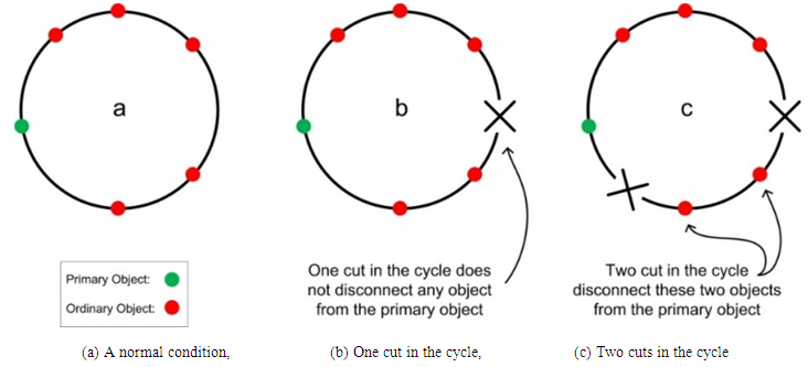 | Figure 1. A cycle connects a primary object with a number of ordinary objects |
Based on this, it is obvious that the reliability of a path is related to the length of the risky parts as well as the number of objects which are lost in case of a cut in those parts. Therefore, the measure for reliability which is called risk of failure is formulated based on these factors, i.e. length of the risky parts and the number of objects. The risky path of a cable cycle is either inevitable or intentional. The former is valid when the configuration of objects and routes does not allow to avoid some risky paths even in return for a longer path due to objects on dead-ends or parallel objects, as depicted in Figure 2. The latter takes place when risky paths are taken for the sake of a path shortening, see Figure 3. However, since risky paths reduce the reliability of systems, it should be decided whether it is worth considering them in return for a shorter path. Note that higher reliability does not always contribute to extended lengths but in most cases does. Therefore, it is often required to strike a compromise between the length and reliability to obtain a reasonable solution.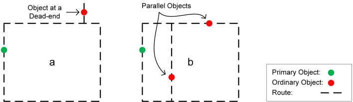 | Figure 2. Inevitable risky path: (a) An object located on a dead-end, (b) Two parallel objects make it impossible to have a perfect cycle solution |
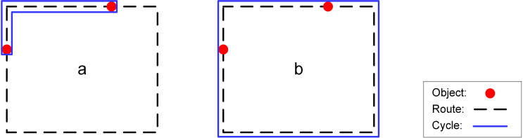 | Figure 3. Intentional risky path: (a) A Cycle with risky path, (b) A Cycle without risky path |
The problem addressed in this work is considered to be NP-hard as there are similar intractable problems, such as the problem of order-batching in a warehouse [1], which are reducible to the current problem and have been proven to be NP-hard. As a consequence a naïve brute-force search for identifying potential candidates is impractical in solving this problem [2].An approximate search algorithm such as Simulated Annealing [3] [4] cannot solve the problem due to two main reasons. The first reason is that the problem is not transformable as a TSP case, because some of the paths between pairs of objects which are not the shortest ones will be missed during a transformation. Those paths might be useful in forming a cycle which will be desirable as a solution. The second reason is that reproducing sequences of nodes representing a valid cycle will not be deterministic in a random manner due to the graph which is not fully connected and includes optional nodes. Therefore, a random search based on such a reproduction will be uncontrollable and so to say, it becomes a blind search.The main contribution of this work is to propose a two-stage search mechanism to solve the cable routing problem. In the first stage, the shortest path is found between every pair of required nodes using the Dijkstra’s shortest path algorithm [5]. This will form a graph in which every node is required and the edges represent the shortest path and distance between them. The graph is then fed into a Simulated Annealing algorithm to find a near shortest solution. The properties (length and risk) of that solution are invoked to set bounds during an exact search in the second stage. In order to have that search efficient and practical, four novel techniques are proposed and tested in the second stage. One of the most effective techniques is using a new kind of directed graph to perform a guided search. This special graph is produced by analyzing the preliminary graph and labeling its nodes. Those labels help to prevent invalid and unreasonable solutions in a search. Another technique which is effective in speeding up the search is heuristic length estimation of future solutions which are derived from a current partial solution. The other two techniques are two different validation tests. The first is to reject any partial cycle with loops which do not include any required nodes and the second one is to reject any unreasonable solution. This rest of this paper is organized as follows. In Section 2, the literature review is presented. Section 3 presents the length-risk model. In Section 4, the proposed techniques are presented and tested. Results and discussions are elaborated in Section 5 and in Section 6 conclude the paper.
2. Related Work
From literature survey and to the best of the knowledge of authors, the problem addressed in this paper is seemingly not taken up by researchers thus far. This section presents some of the works which are loosely related to the current work. Wasem [6] proposed a two-stage algorithm for solving a particular ring network design problem. The author also discussed dissimilarities of that problem with the TSP. Since these dissimilarities are also true for the current problem, they are mentioned briefly below:• The classical TSP deals with a complete graph, while in most variation of ring routing problem the graph is sparse.• A cycle or tour in the TSP includes all the nodes of graph, whereas in most ring routing problems, some of the nodes are only required (the rest are optional). • In the TSP, the objective is to find a tour with a minimum cost (e.g., length), but that type of solution may not be technically appealing in a ring routing problem.Fink et al. [7] studied the similarities in different ring network design problems and produced a general problem formulation. They also presented the application of meta-heuristics to some ring network design problems. They claimed that the General Ring Network Design Problem (GRNDP) covers a great variety of combinatorial optimization problems with a ring-like structure. However, there are many other ring network design problems which were not considered in their work.Laporte et al. [8] proposed a method to solve the Selective Travelling Salesman Problem. The problem is maximization of total profit with cost (i.e., length) lower than a preset value. Every inclusion of nodes in the cycle solution increases the total profit, but it can also increase the cost. The approach for solving the problem consists of finding lower and upper bounds by approximate algorithms and exploiting them in an exact algorithm using a branch-and-bound.Cornuéjols et al. [9] considered a variant of the classical TSP calling “the Steiner Travelling Salesman Problem”. The goal in Steiner TSP, same as the classical TSP, is to minimize the tour length, but visiting some of the nodes is not mandatory. Moreover, unlike the classical TSP, nodes and links could be included in a tour more than once. There are also problems which are classified as a Steiner TSP, such as the problem of order-picking in a warehouse [10] [11] [12] and the Steiner Ring Network Design Problem [13].As cited in [9] [14] [13], an instance of the Steiner TSP could be transformed into an instance of the standard TSP by calculating the shortest path between every pair of required nodes. Other than the disadvantages of the transformation [9], it is not applicable for some variants of the Steiner TSP such as the current problem.
3. The Length-Risk Model
Prior to description of the problem and the solution proposed, the definition of different types of cycles and nodes used are given in the following. • Shortest cycle: It is a cycle which connects all of the objects in the shortest possible way with any value of risk. A shortest cycle is optimal from the financial point of view.• Most reliable cycle: It is a cycle which connects all of the objects with the minimum risk of failure. Note that the risk of the most reliable cycle is not necessarily zero (i.e., 100% reliable), but sometimes it is. The length of the most reliable cycle can either be equal to or more than the shortest cycle and it is optimal from the technical point of view.• Ideal cycle: It is the shortest cycle with a risk equivalent to that of the most reliable cycle. In many cases, this cycle may not exist.• Most reasonable cycle: It is a cycle which connects all of the objects with properties as close as possible to an ideal cycle. There is also a parameter, called Acceptable Extra Length (AEL, determined by the company), which does not allow the length of the most reasonable cycle to be more than a certain amount longer than the shortest cycle’s length. Obviously, the risk of a most reasonable cycle cannot be more than the shortest cycle’s risk.In addition to the cycles, there are two types of nodes are present in the graph:• Required nodes representing the objects (one of the required nodes is a primary node which represents the primary object).• Optional nodes representing the intersections or the end points of the routes.Since a required node represents an object, it must be included in a cycle solution in any condition; while an optional node could be missed in a cycle when the inclusion of the node only increases the cost (i.e., length or risk).An edge of the graph is a route segment between two nodes of any type. That is, a route can be segmented into weighted edges based on the number of objects and the intersections it contains. The weight of an edge is the geometrical distance between two nodes which are linked by that edge. Figure 4 illustrates a simple case transformation in which Figure 4a shows a two-route structure including one object and Figure 4b is the corresponding transformed graph.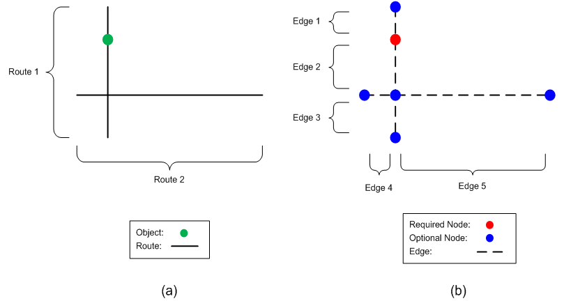 | Figure 4. Illustration of (a) routes and object as well as (b) the corresponding graph |
The length-risk plot depicted in Figure 5 represents the milestone of the length-risk model. The properties of the candidates considered in the search fall in a specific area in the length-risk plot. This area is specified by the risk of the most reliable cycle (rmrl), the risk of the shortest cycle (rsh), the length of the shortest cycle (lsh), and the value of AEL (le). This area is trapezoidal in shape as in Figure 5, and this represents the search area. A line drawn from (rsh ,lsh) which intersects the upper limit of the length will specify the search area. The slope of the line indicates the importance of the risk to the length. This means the amount of compromise between the risk and length is equal by all the solutions which are located on this line. A slope of -1 means that the length and the risk are equally important while a slope [0,-1} gives more importance to the risk while a slope less than -1 gives more importance to the length.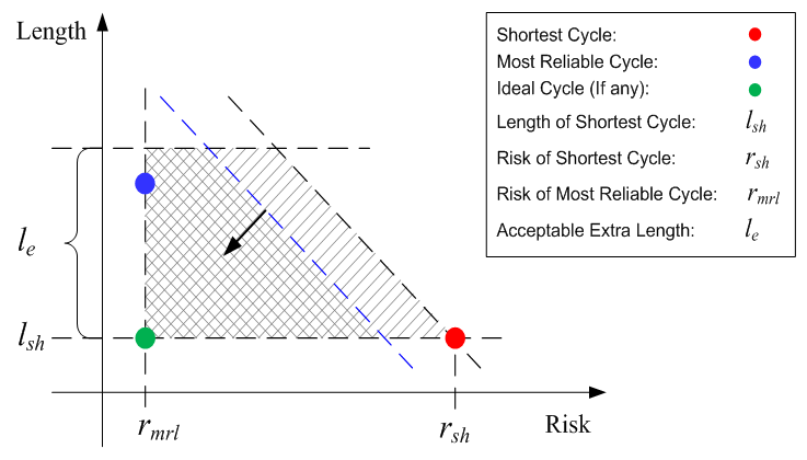 | Figure 5. A length-risk plot for showing the area which is searched for a solution |
In the beginning of the search, the blue line and the black dashed line lie upon each other. As the search proceeds, the blue line moves toward a possible ideal cycle (i.e., the green dot), with the same slope, and the double hatched trapezoid becomes smaller gradually. In case that an ideal cycle does not exist, the line stops somewhere in the middle of the bigger hatched trapezoid (which means there will not be better solutions after that point). The blue line at that moment will be an indicator for the properties of most reasonable solution(s). Obviously, in case an ideal cycle exists, the blue line reaches the green dot which means the ideal cycle will be the solution. Given a graph G which consists of a set of edges E and a set of nodes N, the nodes in this graph should consists of one primary node, a number of required nodes, and a number of optional nodes. A valid cycle VC is a path that starts from the primary node, visits each of the required nodes at least once and returns to the primary node at the end without visiting any edge more than twice. Such a cycle may contain none or any number of the optional nodes, once or more. Therefore, a shortest cycle in a graph can be defined as a valid cycle which minimizes the length. The length function for VC is given in Eq. 1, 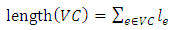 | (1) |
where the length of an edge e is denoted by le.In this case, VCi will be the shortest cycle if: | (2) |
Now to formulate the risk, first, a risky edge in VC is defined by:if  with occurrence(e) = 2, e would be a risky edge.Also, a loss function for VC is defined such that
  returns the number of required nodes (i.e., the objects) which will be lost if erisky is disconnected. In order to decide the reliability of VC, the length and the loss function are invoked to compute the risk function which is defined as follows:
 | (3) |
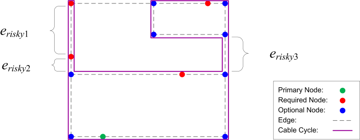
where RE is the set of all risky edges in VC such that  .The unit of a measured risk is mO, where m is the length in meters and O is the object.In order to illustrate this concept, the risk of the valid cycle depicted in Figure 6 is calculated. The cycle links a primary node and four required nodes, containing three risky edges. First, the number of lost required nodes is decided independently for every risky edge (while assuming the edge is cut), as follows:
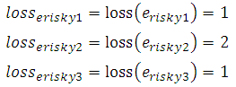
 | Figure 6. Example of a valid cycle with three risky edges |
By using Eq. 3, the risk of the example in Figure 6 is calculated as follows: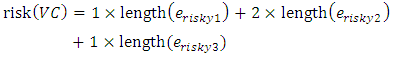 In order to minimize the cost, the main constraint to deal with is the extra length of cable above the actual length required for the shortest cycle. For every instance of the problem, the amount of extra length is determined by the AEL parameter (lextra). This extra length specifies the upper bound of the length of the cable. While the lower bound of the length (llb) is specified by the length of the shortest cycle, the upper bound (lub) is determined by adding the extra length to that of the lower bound. In addition, the risk of a shortest cycle will be specified by the upper bound of the risk (rub), because any cycle with a risk greater than a shortest cycle’s risk cannot be a reasonable solution since it will be longer than the shortest cycle. The lower bound length, the upper bound length, and the upper bound risk are given by Eq. 4-6:
 | (4) |
 | (5) |
 | (6) |
where SHC is a shortest valid cycle.Since it is required to have evaluation criteria for deciding whether a valid cycle is reasonable, ratios (based on the risk and length factors) are defined to indicate deviation of a candidate cycle from a shortest cycle (which is an economical solution) and be used for ranking candidates. So, a length ratio lrvc, a risk ratio rrvc and an overall ratio orvc for a valid cycle VC are defined in Eq. 7-9: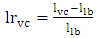 | (7) |
where 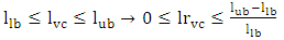
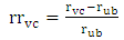 | (8) |
where 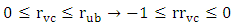
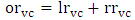 | (9) |
where  Based on Eq. 9 a valid cycle VCi will be the most reasonable if the inequality given by Eq.10 is satisfied:
 | (10) |
That is, the most reasonable cycle is the valid cycle with the minimum overall ratio.
4. The Proposed Method
The proposed method as depicted in Figure 7, starts by transforming the raw data represented by the 3D coordinates of the objects and routes positions into an initial graph (G). The initial graph consists of the nodes and edges without any directions. It is transformed into a Hamiltonian graph (HG) which is used in the initial search. The transformation from the G graph into the HG graph, Figure 8, is achieved by finding the shortest path between every pair of the required nodes by applying Dijkstra’s algorithm. The length of every shortest path, which is called the shortest distance, is simply determined by adding up the length of all edges the path consists of. This forms a graph in which the nodes are considered as required nodes and the graph edges represent the shortest distance between them. The resulting HG is employed in a search to find the shortest cycle which is needed to decide the bounds (Eq. 4-6). Since finding the shortest cycle itself is NP-hard, a simulated annealing algorithm (SA) is used as an approximate search. This approximate search is invoked to find a near the shortest cycle because such a search is impractical to solve the whole problem. The transformation from the graph G into the HG was essential because it was invoked by the SA to find near the shortest cycle. As soon as the near the shortest cycle is specified, its length and risk are calculated in order to decide the aforementioned bounds which are passed as one of the inputs parameters of the final exact search.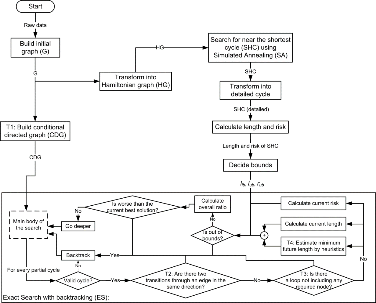 | Figure 7. Block diagram of the proposed method |
 | Figure 8. Transformation of (a) an original graph of the problem to (b) a Hamiltonian graph, based on the shortest path between the required nodes |
The graph G is transformed into a novel type of graphs called a conditional directed graph (CDG). CDG is one of the techniques employed to reduce the search time which is referred to as Technique 1. By a CDG, a number of improper returns are excluded from the path of a cycle and the search which leads to unreasonable solutions is prevented. The difference between a CDG and a typical directed graph (digraph) is that the directions between the nodes are flexible in a CDG, while they are certain in a digraph. Conditional directions in the CDG are defined such that moving from one node to another requires checking the previously traversed node. Such a definition depends on the nodes’ type, geometrical position, and topology.A return in a path is defined as a transition from a current node to a previously traversed node. There are three types of returns which leads a cycle to be an unreasonable solution and conditional directions help to avoid them:1. Any return at an optional node2. Particular returns at required nodes on a branch which is defined as a path between two branchy nodes (Branchy node is a node with degree more than two or  ) without any other branchy node in between.3. Particular returns at required nodes on a dead-end path (Dead-end node (leaf) is a node with degree 1 or
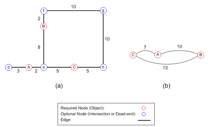
  ) which is a path between a branchy node and a dead-end node without any other branchy node in between.The first type of returns (return type 1), which is a simple return at an optional node, will only increase the length of a cycle without linking any new required node. Removing such a return from a cycle will result in a new cycle. The new cycle will have a shorter length and the same risk compared to the cycle including the return.The second type of returns (return type 2) takes place under certain circumstances at required nodes on a branch which contains at least two required nodes. The number of the required nodes is counted in the whole branch. It includes the two nodes at the two ends if any of them is a required node, Figure 9a. For a certain edge ec between two required nodes in such a branch, a common path is the common part (not out of the branch) of the path of the valid cycles which do not include ec. The common length
  and the common risk
  which are length and risk of that path for ec are given by Eq. 11 and 12, respectively, where B is the set of all edges of the branch under consideration:
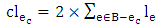 | (11) |
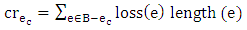 | (12) |
The common cost  for the edge ec is given by Eq.13:
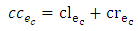 | (13) |
The best gap in a branch with more than one required node is an edge which has minimum cc in the branch, Figure 9a. The unwanted returns will be specified by the two nodes of the best gap as well as the first and the last required nodes of a branch. The returns which are suppressed are: 1. All nodes of a branch before the first node of the best gap2. All nodes between the first node of the best gap and the last required node of a branchThe final conditional directions defined on the branch are shown in Figure 9b. Every sign in the figure consists of a dotted line and arrow(s). In any node in the branch, the dots represent the direction from where the exploration takes place, while the arrows represent the possible direction of continuations. A return at a last required node (based on the direction of movement) should not be suppressed, because a branch might be the only way for traversing from one of the two end nodes of the branch to another.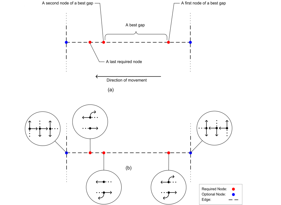 | Figure 9. Illustration of a branch: (a) Different types of nodes, (b) Conditional directions and suppression of type 2 returns |
The last type of returns (return type 3) happens in two different situations in a dead-end path. The first situation is when early returns happen at a required node before connecting the rest of required node(s) in a dead end, as in Figure 10a. The other situation happens when a dead-end path is explored toward the exit node and a return takes place at any of the required nodes closer to that exit node. This situation is illustrated in Figure 10b when the exploration goes from node 2 to 1 and then instead of continuing to the exit node it returns back to node 2. Thus, any of such returns is not allowed when conditional directions are defined for a graph.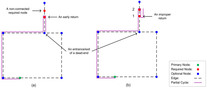 | Figure 10. Returns in a dead-end path leading to invalid cycles |
All the three types of the returns are prevented in the final search by defining similar signs to those illustrated in Figure 9b for all nodes in the graph G. The resulting graph, which is a CDG, is explored in the second stage search for the most reasonable and most reliable solutions.The exploration starts from the primary node and partial cycles are generated and expanded by including new nodes in a depth-first order. For every node included in any partial cycle, different validations and evaluations are performed in order to decide whether the corresponding node is accepted or rejected. In case of the acceptance, the search goes one stage deeper, while in case of rejection it backtracks to a previous state.The first validation test is based on the definition of valid cycle. Every inclusion of a node which leads to a partial cycle to go through an edge more than twice is rejected.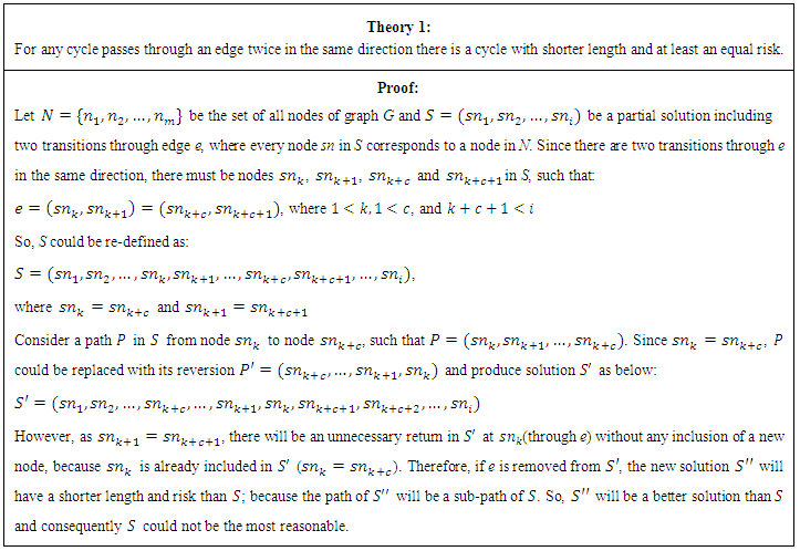 The second validation test (Technique 2) is designed to reject partial cycles which go through an edge twice in the same direction according to Theory 1, as illustrated in Figure 11. Those partial cycles lead to unreasonable complete cycles. Therefore, rejecting those partial cycles makes the search faster. Hence, as soon as such a transition is detected in a partial cycle, a backtracking could be done from that state. This helps to prevent any further exploration from that state and ensures faster search.
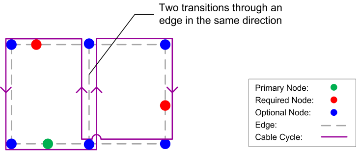 | Figure 11. Two transitions through an edge in the same direction |
The last validation test, which is called Technique 3, is for rejecting partial cycles with loops which do not include any required nodes (see, Figure 12). It reduces the search time by employing an early detection mechanism of partial cycle with loop(s), which does not contain at least one required node, from the set of all partial cycles.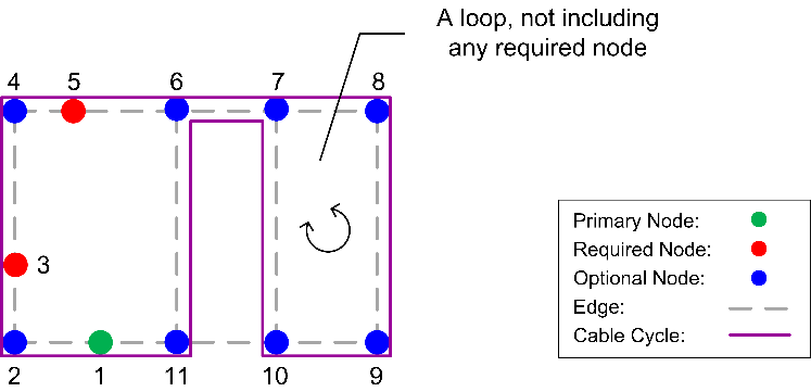 | Figure 12. A cycle with a loop not including any required node |
A loop in a path is recognized when at least one node is visited twice during the exploration of that path. Figure 12 illustrates a situation where nodes 6 and 7 are visited twice during this exploration.A cycle with a loop not containing any required node could not be reasonable because it will contain a cycle with shorter length and the same risk. To prove this concept, let  be a solution containing a loop with no required nodes which occurs between two occurrences of node n. A solution
  which is shorter than
  (because
  ) with the same risk can be reached by removing all the nodes between the two occurrences of n and merging them into one. Hence,
  could not be most reasonable because a partial cycle containing such a loop is detected and an early backtracking makes the search more efficient.To illustrate that any partial cycle with such a loop does not lead to a reasonable solution refer to Figure 12. The nodes 1, 2, 3, 4, 5, 6, 7, 8, 9, 10, 7, 6, and 11 in the demonstration cycle are visited starting from primary node and back to this node. It is clear that node 6 is visited twice. Since all the nodes between the two occurrences of node 6 are optional nodes, this part of the cycle will generate a loop consisting of nodes 7, 8, 9, and 10 which neither of them is a required node. In this case, it is obvious that the cycle which consists of nodes 1, 2, 3, 4, 5, 6, and 11 does not contain such kind of loop and, therefore, it will be a better solution.The evaluation process starts immediately after the validation process and exploits an admissible heuristic (Technique 4) to detect and reject partial cycles leading to unreasonable earlier solutions. It is based on the current length and risk of a partial cycle as well as the heuristic which estimates the minimum possible length of complementary paths which converts the partial cycle into a complete one. A complementary path links together the partial cycle’s head and tail points as well as any remaining required nodes which are not connected with that partial cycle. For every partial cycle, a minimum possible length of all complementary paths can be decided first by calculating two Manhattan distances between the end points of any partial cycle and every remaining required node (see, Figure 13). The Manhattan distance is calculated using the 3D coordinates of the corresponding nodes. These two Manhattan distances are then summed up together, for every remaining required node separately. A sum with the greatest value among others will represent the lower bound for the length of all complementary paths. Moreover, the outcome is summed up with the current length of a partial cycle to result in a lower bound for the total length of any complete cycle derived from that partial cycle. For partial cycles which already link all required nodes, the lower bound of the complementary path will be the Manhattan distance between the two end points of the partial cycles.
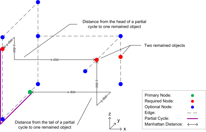 | Figure 13. Measuring Manhattan distances for heuristic length estimation of final cycles derived from a partial solution |
In the current state, a partial cycle under consideration is rejected if either of the following two conditions is true:• The current risk of the partial cycle > The risk upper bound (rup)• The current length of the partial cycle + The value of estimation > The length upper bound (lup)In the next state of the evaluation, the overall ratio of the partial cycle (based on the current risk and the estimated length) is calculated and compared with the overall ratio of a current best found solution. A partial cycle which has greater overall ratio than the best solution is rejected. Otherwise, it will be kept for further expansion. Moreover, the best solution will be replaced by any partial cycle which is not rejected and becomes a complete valid cycle. This process is repeated until all the CDG is explored.
5. Results and Discussions
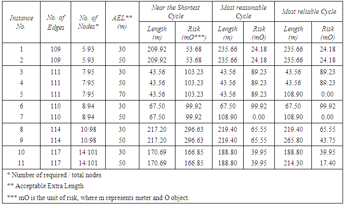
The dataset employed in this work consists of 3D positions of objects and routes in a ten-story power plant building. Five sets of objects were selected to test the proposed method. They consist of 5, 7, 8, 10 and 14 objects which are independently connected by different cable cycles routed through a set of 78 horizontal and vertical routes. By setting different values for the AEL parameter, 11 different instances were created as listed in Table 1. All sets of objects except the one with 7 objects were tested with two different values of the AEL. The set with 7 objects was tested with three different AEL values. This variation in the AEL was essential to study the effect of the extra length on the quality of the solutions as well as the relative computation time. Three different types of cycles, namely near the shortest cycle, the most reliable cycle, and the most reasonable cycle were computed for each instance. In addition to the fact that obtaining the near the shortest cycle was essential to find the other two types of cycles, it is invoked as a reference when comparing the other two types of cycles. Table 1 depicts the properties (length and risk) of the three aforementioned cycles of the 11 instances. Table 1 also includes the number of edges and nodes of each instance as well as the values of the AEL parameter. The dashed lines in the table separate the instances with different configuration of objects.According to Table 1, two or all of the three types of cycles are identical for some of the instances either due to the arrangement of required nodes, or because of the value of the AEL. For instance, all the three types of cycles of instance 6 are the same because AEL does not allow a cycle to be 30m longer than the near the shortest cycle. When this parameter is increased to 50m for the same set of required nodes (instance 7), the most reasonable and reliable cycles start to differ from the near the shortest one. Since an increment of the AEL from 50 to 70m does not provide any more changes in the solutions for the 1st, 3rd, 4th and 5th sets of instances (due to the arrangement of their required nodes), the result of such increment for the 2nd group is only presented. Also note that increasing the AEL from 30 to 50m in set 5 leads to a longer but more reliable cycle.Table 1. Cycle properties (length and risk) of the near the shortest cycle, the most reasonable cycle, and the most reliable cycle
 |
| |
|
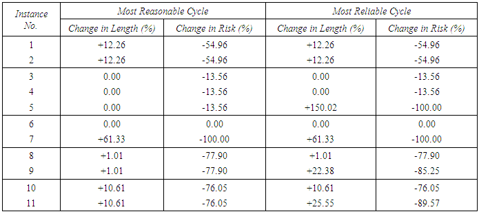
Although by increasing the value of the AEL one allow a cycle to be longer and the run-times increases, but nevertheless, in return a lower risk is gained. Moreover, for practical reasons, solutions which are very much longer than the shortest one are eliminated even if the solution does not give any risk. Thus, the search always starts with a small value of AEL and then increase it to larger values if the solution is not satisfactory.Since a near the shortest cycle is considered as a good solution from financial point of view, calculating the deviation of the length and risk of the other two types of cycles helps to evaluate a most reasonable solution. Table 2 illustrates those deviations which represent the trade-off between length and risk. In this table, increasing the length of most reasonable cycle of instance 1 by 12.26% will reduce the risk by 54.96%, for instance. In order to give a better picture to the amount of win in the risk and loss in the length of the most reasonable and reliable solutions compared to the near the shortest ones solutions, the data in Table 2 is plotted in Figure 14 and 8, respectively.Table 2. Amount of change in length and risk of the most reasonable and most reliable cycles compared to corresponding near the shortest cycles. The + sign means increment in the length, while the - sign means decrement (improvement) in the risk
 |
| |
|
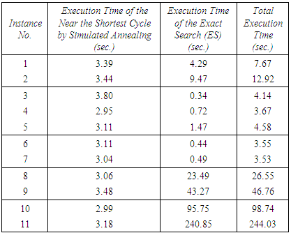
Table 3. Execution Times of the searches for the solutions
 |
| |
|
According to Figure 14, the most reasonable solutions can be categorized into four groups. The first group comprises solutions of instances 1, 2, 8, 9, 10 and 11. With the cost of a little longer cable length compared to the near the shortest solutions the risk is considerably reduced. The solution of instance 7 falls in another group which removes the risk completely, but the increment in length is not as low as the previous group. While the compromise between length and risk in the two aforementioned groups is not very far from the expectation, the solutions in the two other groups might look a little odd. The solutions of instance 3, 4, and 5, which are in one group, decrease the risk by 13.56% without any increment in length. To explain how it is possible to decrease the risk without increasing the length, a reference to the objects and routes is essential. For a set of objects and routes there might be several shortest paths (with equal length) between two objects. In the approximate search for a near the shortest solution, only one of those paths is considered (stochastically), while in the search for a most reasonable solution all of them are taken into account. The last group contains the solution of instance 6 which is not better than the near the shortest one. The reason is that the arrangement of the objects and the limit which is the preset of AEL do not allow any improvement in risk. 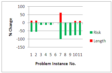 | Figure 14. Illustration of the changes in length and risk of most reasonable cycles compared to the corresponding near the shortest cycles |
Figure 15 depicts that the risks of the most reliable solutions of instance 9 and 11 are improved more than the corresponding most reasonable instances (~85-90% compared to ~76-78%). However, as it is expected, the amount of length they increase is not as low as what the most reasonable ones do (~22-26% compared to ~1-11%). For the problem instance 5, the amount of increment in length is even much higher. By 100% improvement in risk the length increases by 150.02%. Although the most reliable solutions are not the financially desired ones, they are technically of interest as they might remove the risk completely, which is illustrated by the solution of instance 5. 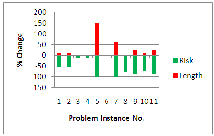 | Figure 15. Illustration of the changes in length and risk of most reliable cycles compared to the corresponding near the shortest cycles |
In order to demonstrate the effectiveness of the proposed solution, run-times of the different problem instances are computed. The run-times were measured on a machine with an Intel® Core™ 2 Duo 2.10 GHz processor, 3.00 GB RAM. In this context, the run-times of the simulated annealing process to obtain a near the shortest cycle, and the run-times of the exact search (ES) to obtain both the most reasonable and most reliable cycles were measured separately. Table 3 depicts these run-times.The results show that the run-times are highly related to the number of nodes, number of edges in each instance, as well as the value of the AEL parameter. Different run-time patterns could be observed for some of the instances. That is, the run-time for some of the instances is more than some that of other instances with higher number of nodes or edges. For example, the run-time for the problem instance 1 (with 5 required nodes and 109 edges) is 4.2 seconds, while it is 0.44 seconds for problem instance 6 (with 8 required nodes and 110 edges). The reason for this difference is that the run-time depends on not only the topology of a graph, but also the geometry of the components of a graph. This means, the run-time of an instance in which all required nodes are close to each other could be shorter than another instance with the same number of required nodes and edges but some or all of its required nodes are far from each other. This could easily be observed for problem instance 1 and 6 by looking at the length of their near the shortest cycles in Table 1.To test the integrity of the proposed techniques, their effectiveness on the solution, and how much they speed up a brute-force search, new tests were performed in which every time one of the proposed techniques was excluded and a measurement was performed with the other techniques. A total of 44 new tests were performed for the 11 instances under consideration. Figure 16 illustrates the result of the tests (run-times) along with the run-times when all the techniques are engaged.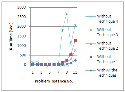 | Figure 16. Illustration of the excecution times for obtaining solutions (most reasonable and reliable) with/without exploiting all/each of the proposed techniques |
It is obvious that the search becomes slower for most of the instances when one of the techniques was excluded. However, it becomes a bit faster for some of the smaller instances when technique 2 is excluded. This is obviously due to the computational burden of the technique. The growth in run-times is more obvious for the instances with a greater number of nodes. It is important to know that excluding all of the proposed techniques causes a vast increment in the run-time of the searches which is not equivalent to the sum of the increments when every technique is separately excluded. Performing such kind of tests for all instances is cumbersome and very time-consuming. Such a test for a small instance with 41 edges, 26 optional nodes, 10 required nodes and setting 30m for the AEL parameter requires a runtime of 2874.71 seconds compared to 0.9 seconds when all the techniques were exploited.
6. Conclusions
This work dealt with a cable cycle routing problem to connect a set of objects through a given set of routes. Both financial and technical concerns were required to be taken into consideration when dealing with this problem. Hence, length and risk factors were the two factors to evaluate the effectiveness of any routing cycle. Due to technical concerns, testing approximate algorithms or finding cycles of subsets of objects and merging them together did not lead to a good solution. The exact search algorithm exploited an approximate one such as Simulated Annealing to set bounds of the solutions. A depth-first search strategy was taken with a sophisticated backtracking approach. Moreover, a new kind of a graph was developed due to the fact that many invalid and non-reasonable solutions could be detected in the middle of a search. The graph could be considered as one of the prominent parts of the work. To prepare such a graph and do a guided search, signs and conditional directions are added to the nodes of an original undirected graph of the problem. Using those directions and signs helps avoid further expansions of undesired partial solutions and have lesser computations in the validation process. A heuristic approach was proposed to estimate the minimum possible length of solutions which are derived from a partial solution. The search tree could be pruned considerably by this heuristic approach. The method was tested for 11 instances. The result depicted that the method could provide satisfactory solutions to the problem within reasonable amount of time. It was also clear that the proposed techniques could reduce the search-space effectively and could make a brute-force search possible for problems with similar scale. Other problems with similar properties can be solved by the proposed techniques due to the effectiveness in reducing the search run-time. For example, the conditional directions as well as the other techniques introduced in the work seem to be also useful in solving larger instances of the order-picking problem in a warehouse to optimum. Also, the method of using an approximate algorithm in setting bounds for an exact algorithm might be a good idea in solving larger instances of problems like the TSP, to optimum. Moreover, the introduced heuristic length estimation might be tested for variety of routing problems.
References
| [1] | N. Gademann and S. Velde, "Order Batching to Minimize Total Travel Time in a Parallel-aisle Warehouse," IIE Transactions, vol. 37, no. 1, pp. 63-75, 2005. |
| [2] | G. J. Woeginger, "Exact Algorithms for NP-Hard Problems: A Survey," in Combinatorial Optimization — Eureka, You Shrink!, vol. 2570, Springer Berlin Heidelberg, 2003, pp. 185-207. |
| [3] | S. Kirkpatrick, C. D. Gelatt and M. P. Vecchi, "Optimization by Simulated Annealing," Science, vol. 220, no. 4598, pp. 671-680, 13 May 1983. |
| [4] | V. Černý, "Thermodynamical Approach to the Traveling Salesman Problem: An Efficient Simulation Algorithm," Journal of Optimization Theory and Applications, vol. 45, no. 1, pp. 41-51, 01 01 1985. |
| [5] | E. Dijkstra, "A Note on Two Problems in Connexion with Graphs," Numerische Mathematik, vol. 1, no. 1, pp. 269-271, 01 12 1959. |
| [6] | O. Wasem, "An Algorithm for Designing Rings for Survivable Fiber Networks," Reliability, IEEE Transactions on, vol. 40, no. 4, pp. 428-432, 1991. |
| [7] | A. Fink, G. Schneidereit and S. Voß, "Solving General Ring Network Design Problems by Meta-Heuristics," in Computing Tools for Modeling, Optimization and Simulation, Springer US, 2000, pp. 91-113. |
| [8] | G. Laporte and S. Martello, "The Selective Travelling Salesman Problem," Discrete Applied Mathematics, vol. 26, no. 2-3, pp. 193 - 207, 1990. |
| [9] | G. Cornuéjols, J. Fonlupt and D. Naddef, "The Traveling Salesman Problem on a Graph and Some Related Integer Polyhedra," Mathematical Programming, vol. 33, no. 1, pp. 1-27, 1985. |
| [10] | H. D. Ratliff and A. S. Rosenthal, "Order-Picking in a Rectangular Warehouse: A Solvable Case of the Traveling Salesman Problem," Operations Research, vol. 31, no. 3, pp. 507-521, 1983. |
| [11] | R. d. Koster, T. Le-Duc and K. J. Roodbergen, "Design and Control of Warehouse Order Picking: A Literature Review," European Journal of Operational Research, vol. 182, no. 2, pp. 481-501, 2007. |
| [12] | C. Theys, O. Bräysy, W. Dullaert and B. Raa, "Using a TSP Heuristic for Routing Order Pickers in Warehouses," European Journal of Operational Research, vol. 200, no. 3, pp. 755-763, 2010. |
| [13] | G. Laporte and Y. Nobert, "Finding the Shortest Cycle through K Specified Nodes," Congressus Numerantium, vol. 48, p. 155–167, 1983. |
| [14] | B. Fleischmann, "A Cutting Plane Procedure for the Travelling Salesman Problem on Road Networks," European Journal of Operational Research, vol. 21, no. 3, pp. 307-317, 1985. |
| [15] | A. N. Letchford, S. D. Nasiri and D. O. Theis, "Compact Formulations of the Steiner Traveling Salesman Problem and Related Problems," European Journal of Operational Research, vol. 228, no. 1, pp. 83-92, 2013. |
 Abstract
 Reference
 Full-Text PDF
 Full-text HTML