Takafumi Sasakawa1, Jun Sawamoto2, Hidekazu Tsuji3
1Department of Science and Engineering, Tokyo Denki University, Saitama, Japan
2Department of Software and Information Science, Iwate Prefectural University, Iwate, Japan
3Department of Embedded Technology, School of Information and Telecommunication Engineering, Tokai University, Tokyo, Japan
Correspondence to: Jun Sawamoto, Department of Software and Information Science, Iwate Prefectural University, Iwate, Japan.
| Email: |  |
Copyright © 2014 Scientific & Academic Publishing. All Rights Reserved.
Abstract
In an ordinary artificial neural network, individual neurons have no special relation with an input pattern. However, some knowledge about how the brain works suggests that an advanced neural network model has a structure in which an input pattern and a specific node correspond, and have learning ability. This paper presents a neural network model to control the output of a hidden node according to input patterns. The proposed model includes two parts: a main part and control part. The main part is a three-layered feedforward neural network, but each hidden node includes a signal from the control part, controlling its firing strength. The control part consists of a self-organizing map (SOM) network with outputs associated with the hidden nodes of the main part. Trained with unsupervised learning, the SOM control part extracts structural features of input space and controls the firing strength of hidden nodes in the main part. The proposed model realizes a structure in which an input pattern and a specific node correspond, and undergo learning. Numerical simulations demonstrate that the proposed model has superior performance to that of an ordinary neural network.
Keywords:
Neural network, Self-organizing map, Advanced neural network model
Cite this paper: Takafumi Sasakawa, Jun Sawamoto, Hidekazu Tsuji, Neural Network to Control Output of Hidden Node According to Input Patterns, American Journal of Intelligent Systems, Vol. 4 No. 5, 2014, pp. 196-203. doi: 10.5923/j.ajis.20140405.02.
1. Introduction
The brain has highly developed information processing capability. The artificial neural network (ANN) in extensive use lately is a model that extends functions of a brain nervous system into a simple form in terms of engineering. The ANN has characteristics such as nonlinearity, learning ability, and parallel processing capability. However, common ANNs can perform only a small fraction of all brain functions. Building an advanced ANN model offering performance that is higher than that of a common ANN can be expected from pursuit of a computation style that more closely resembles that of a brain, referring to knowledge therein.Hebb advocates two theories related to fundamental brain functions: Hebbian learning and cell assembly [1]. The latter claims that neurons within a brain build up groups that bear a specific function using the former. Each built-up group does not stand independently: neurons overlapping multiple groups also exist. Then, a specific group is activated according to information received by the brain: each neuron is bound together functionally rather than structurally, performing appropriate processing according to the information that is received [2].Each neuron has specific input information to which it demonstrates a particularly strong reaction. Moreover, the neuron reaction intensity varies according to similarity with information that elicits a strong reaction [3]. This fact suggests that an advanced ANN model has a structure in which an input pattern and a specific node correspond, in addition to learning ability. Nevertheless, no special relation exists between an input pattern and each node in the common ANN.Research results suggest that the cerebellum, cerebral cortex, and basal ganglia respectively perform behavior specialized to supervised learning, unsupervised learning, and reinforcement learning in a learning system within a brain [4]. This knowledge teaches that an advanced ANN model should comprise multiple parts with a different learning system.This paper presents a proposal of a neural network model to control the output of a hidden node according to input signals based on knowledge about the brain described above. It comprises a main part and a control part: The main part maps the input–output relation of an object by supervised learning, whereas the control part extracts the characteristic of an input space by unsupervised learning. The main part has the same structure as the ordinary three-layered feedforward neural network, but the firing strength at each node of its hidden layer is controlled by a signal from the control part. The control part comprises a self-organizing map (SOM) network [5]. The SOM is an algorithm with a close relation to the function of the cerebral cortex. It is suitable for implementing a structure in which an input pattern and a specific node are related. The output of the control part is associated in one-to-one correspondence with the hidden layer node of the main part, and controls the firing strength of the hidden layer node of the main part according to an input pattern. Consequently, the proposed model realizes a structure in which a specific input pattern and a specific node are related. This study assesses the representation capability of the proposed model by simulation.
2. Proposed Model
The proposed model has learning capabilities and has a structure by which an input pattern and a specific node are related. As Figure 1 shows, it consists of two parts: a main part and control part. The main part realizes the learning capability. The control part extracts structural features of the input space and controls the firing strength of each hidden node in the main part.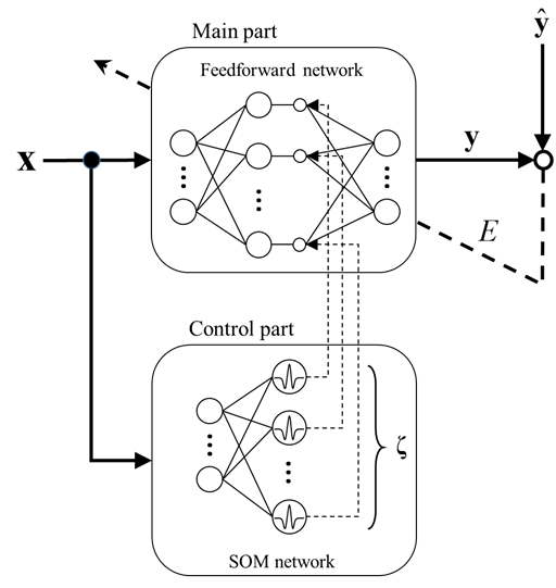 | Figure 1. Structure of the proposed model |
2.1. Main Part
The main part of the proposed model realizes the learning capability to construct an input–output mapping. Structurally, it is the same as an ordinary three-layered feedforward neural network, but each of its hidden nodes contains a signal from the control part, controlling its firing strength.The input vector of the proposed model is  , where
  , the output vector is
  , where
  . The input–output mapping of the proposed model is defined as presented below.
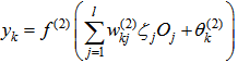 | (1) |
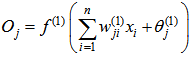 | (2) |
Therein,  and
and  respectively denote the activation functions of hidden and output layers. Also,
  ‘s and
  are the weights of input layer and output layer respectively,
  and
and  respectively represent the biases of hidden node and output node,
  are the outputs of hidden node, l is the number of hidden nodes, and
  is the signal controlling firing strength of hidden node j. It is apparent from (1) that if the firing signal
 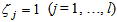 for any input pattern, the main part of the proposed model is exactly the same as an ordinary feedforward neural network. The firing signal vector
 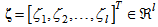 is the output vector of the control part.Similar to an ordinary feedforward neural network, the main part realizes the input–output mapping of the network. However, the firing strength of each hidden node in the main part is controlled by signals corresponding to the output of the control part.
2.2. Control Part
The control part is a SOM network that extracts the structural features of input space and controls the firing strength of each hidden node in the main part. The SOM network has one layer of input nodes and one layer of output nodes. An input pattern x is a sample point in the n-dimensional real vector space, where 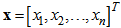 . This is the same as the input to the main part of the proposed model. Inputs are connected by the weight vector called the code book vector
 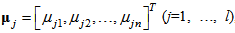 , where l is the total of hidden nodes of the main part, to each output node. One code book vector can be regarded as the location of its associated output node in the input space. There are as many output nodes as the number of hidden nodes of the main part. These nodes are located in the input space to extract the structural features of input space by network training. For an input pattern x, output of the control part is calculated using a Mexican hat function. It is defined as shown below.
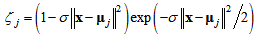 | (3) |
Therein,  stands for the output of the jth node,
  represents a parameter that determines the shape of Mexican hat function.Figure 2 presents an example of the control part output. As shown in Figure 2, each of the output nodes in the control part is associated with one hidden node in the main part. By multiplying the output of each hidden node by the output of the associated node of the control part, the firing strength of hidden nodes is controlled according to the Euclidean distances between the nodes and the given input pattern. When
  the proposed model is equivalent to an ordinary feedforward ANN because all outputs of the control part are equal to 1. In this way, the proposed model relates its hidden nodes with specific input patterns. It is readily apparent that σ is an important parameter for constructing the proposed model. How to determine an optimal value of σ, however, remains an open problem. Further research is needed.
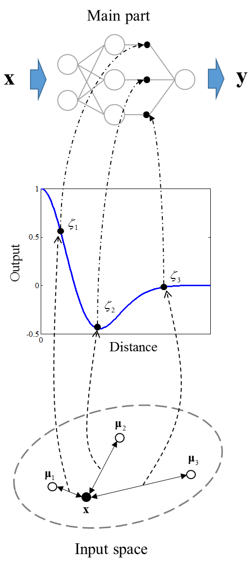 | Figure 2. Example of the control part output |
3. Training of the Proposed Model
Training of the proposed model consists of two steps: an unsupervised training step for the control part and then a supervised training step for the main part.
3.1. Unsupervised Training for the Control Part
A traditional SOM training algorithm is useful for the control part training. The algorithm for SOM network training is based on a competitive learning, but the topological neighbors of the best-matching node are also similarly updated. It first determines the best-matching node, for which the associated weight vector  is the closest to the input vector x in Euclidean distance. The suffix c of the weight vector
  is defined as the following condition.
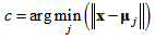 | (4) |
Then, it updates a code book vector  by the following rule.
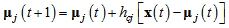 | (5) |
Therein, t denotes the training step and  is a non-increasing neighborhood function around the best-matching node
  . The
. The  is defined as
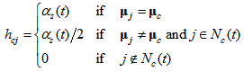 | (6) |
where  is the learning rate function and
  is the neighborhood function for
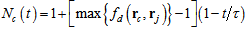
  .SOM training comprises two phases: The ordering phase and the tuning phase. In the ordering phase, each unit is updated so that its topological relation ordered physically and the topology in input space is the same. The learning rate function and the neighborhood function are decreased gradually based on the following rule.
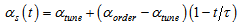 | (7) |
 | (8) |
In those equations,  stands for the learning rate for the tuning phase,
  represents the learning rate for the ordering phase, and
  denotes the steps for the ordering phase. After the ordering phase, a tuning phase is conducted. In the tuning phase, the location of each unit is finely tuned. The neighborhood function is fixed, while the learning rate function decreases slowly based on the following rule.
 | (9) |
 | (10) |
Therein,  is the neighborhood distance for the tuning phase.
3.2. Supervised Training for the Main Part
Because the main part of the proposed model structurally is the same as an ordinary neural network, similar to an ordinary neural network, the training can be formulated as a nonlinear optimization and solved using the well-known back-propagation (BP) algorithm. The nonlinear optimization is defined as | (11) |
where  is the parameter vector and W denotes a compact region of parameter vector space, SSE is the sum of squared errors defined as
 | (12) |
where  stands for the teacher signal and D represents the set of training data.The BP algorithm used to solve the nonlinear optimization (11) is a faster BP that combines the adaptive learning rate with momentum. It is described as
 | (13) |
 | (14) |
where  is the parameter vector of the main part at t training step,
  is the coefficient of momentum term introduced to improve the convergence property of the algorithm,
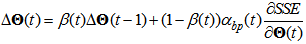
  represents the learning rate that is tuned based on the following rule
 | (15) |
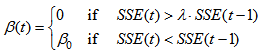 | (16) |
where  and
and  respectively represent ratios to increase and decrease the learning rate, and
  is the maximum performance increase. Furthermore,
  , where
  and
and  in (16) respectively stand for the initial values of learning rate and momentum coefficient.
4. Numerical Simulations
In this chapter, we present some numerical simulations to show that the proposed model has better representation capability than that of an ordinary feedforward ANN.
4.1. Problem Description
We apply the proposed model to benchmark problems: the two-nested spirals problem and the building problem taken from the benchmark problems database PROBEN1 [6].
4.1.1. Two-nested Spirals Problem
The task of the proposed model is to separate the two-nested spirals. The training sets consist of 152 associations formed by assigning the 76 points belonging to each of the nested spirals to two classes using output values 0.1 and 0.9. The problem has been used extensively as a benchmark for the evaluation of neural network training [7].The setting of the main part used for this problem is the following. Number of input nodes: 2 Number of output nodes: 1 Number of hidden nodes: 10The numbers of input and output nodes are values inherent in the problem. The activation functions used in the output nodes and the hidden nodes respectively constitute standard sigmoid and tanh. The number of hidden nodes is the value such that an ordinary ANN with this number of hidden nodes is not able to solve the problem, while the proposed model with proper value of σ can solve the problem. The control part has the same number of output nodes as the number of hidden nodes of the main part. The topology of the output nodes of the control part, or SOM network, is defined in a physical space, as shown in Figure 3.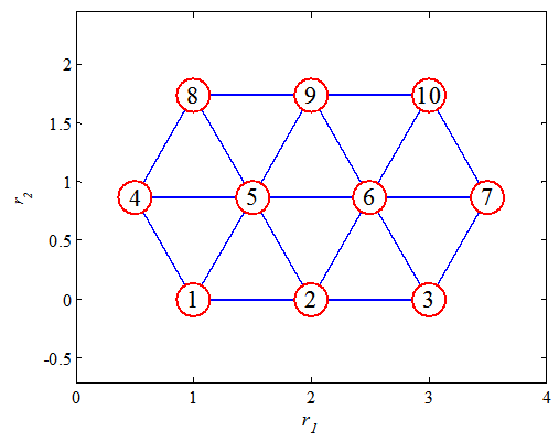 | Figure 3. Neuron positions of the control part defined in a physical space for the two-nested spirals problem |
4.1.2. Building Problem
The purpose of the building problem is to predict the hourly consumption of electrical energy, hot water, and cold water, based on the date, time of day, outside temperature, outside air humidity, solar radiation, and wind speed [6]. This problem has 14 inputs and 3 outputs. In PROBEN1, three different permutations of the building dataset (building 1, building 2, and building 3) are available. Here we use the dataset building1 with 2104 examples for the training set.The setting of the main part used for this problem is the following. Number of input nodes: 14 Number of output nodes: 3 Number of hidden nodes: 100The activation functions for this problem are the same as the section 4.1.1. The topology of the output nodes of the control part is defined in a physical space, as shown in Figure 4.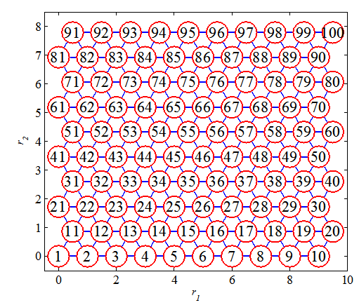 | Figure 4. Neuron positions of the control part defined in a physical space for the building problem |
4.2. Representation Ability of the Proposed Model
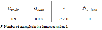
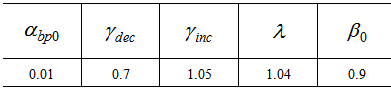
In this section, we shall verify the representation ability of the proposed model. The algorithm described in Chapter 3 is used to train the proposed model.First, the control part is trained for  steps. Note that P is the number of examples in the dataset considered. The conditions used for the SOM training are presented in Table 1. Then the main part with a random initial value is trained. For this training, 300,000 steps and 3,000 steps are used for the two-nested spirals problem and the building problem, respectively. The conditions used for the BP training are shown in Table 2. The value of σ in equation (3) is set to σ = 15 for the two-nested spirals problem and is set to σ = 1 for the building problem. In these simulations, the algorithms for both training Step 1: unsupervised training for the control part and Step 2: supervised training for the main part were modified for our model from those provided in Matlab Neural Network Toolbox [8] [9].
Table 1. Training parameters for SOM network
 |
| |
|
Table 2. Training parameters for BP algorithm
 |
| |
|
To demonstrate that the proposed model has better representation ability than an ordinary ANN, an ordinary ANN that has the same network size as the main part is also trained using the same BP algorithm. Because the BP algorithm easily becomes stuck at a local minimum, we run the same simulations 50 times. For comparison, initial values for both BP training are the same.Figures 5 and 6 respectively present histograms of SSE on the two-nested spirals problem and the building problem. These results were obtained from both the proposed model (blue) and an ordinary ANN (white). In Figs 5 and 6, even the worst result obtained from the proposed model is better than the best result obtained from an ordinary ANN, which shows that the proposed model has superior representation ability with a proper value of σ compared to an ordinary ANN.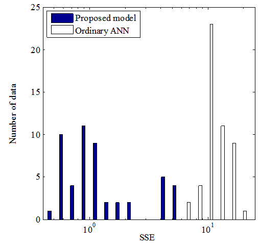 | Figure 5. Histogram of SSE obtained from both the proposed model and from an ordinary ANN on the two-nested spirals problem |
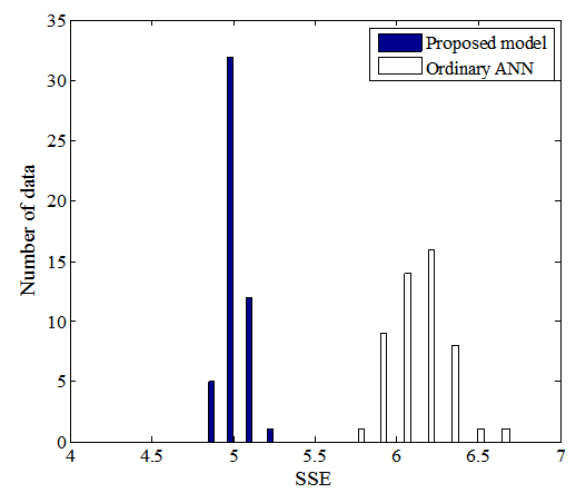 | Figure 6. Histogram of SSE obtained from both the proposed model and from an ordinary ANN on the building problem |
5. Discussion
5.1. Effects of Parameter σ
Here, we discuss how the value of the parameter σ affects the representation ability. To verify the effect of σ on the training, we carry out a set of simulations by varying σ by the same way as section 4.2. For the two-nested spirals problem, we set σ from 0 to 25 at intervals of 5. Also for the building problem, the value of σ is set from 0 to 5 in increments of 1. Figure 7 shows output of the control part when σ = 1, 5, 15, and 25. Output depends on the Euclidean distance between an input pattern x and a weight vector  in the control part.
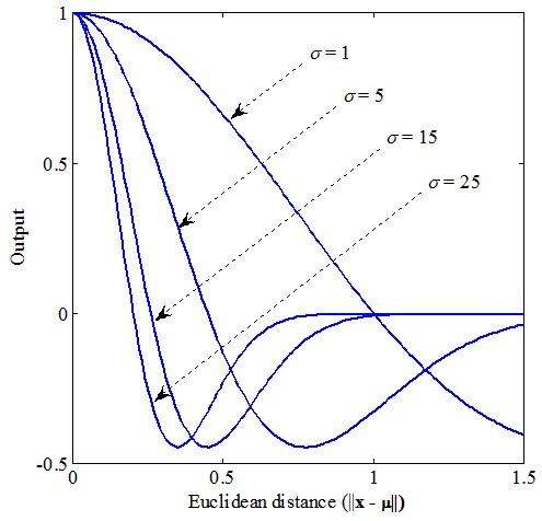 | Figure 7. Output of the control part with different σ |
It is apparent that the range within which the output is 0 becomes wide as the value of σ is increased, in Figure 7. Therefore, the hidden nodes which have some involvement in the output of the main part might increase as σ gets larger. Whenσ = 0 the proposed model reduces to an ordinary ANN because all outputs of the control part are equal to 1. The trained control part and initial values for each set of simulations are the same for comparison.Figures 8 and 9 present results of averaged SSE on the best three runs out of the 50 runs and all runs on the two-nested spirals problem (Fig. 8) and the building problem (Fig. 9). It is apparent that all results obtained from the proposed model have better representation ability than an ordinary ANN (σ = 0). Apparently, too small or too large σ does not work well.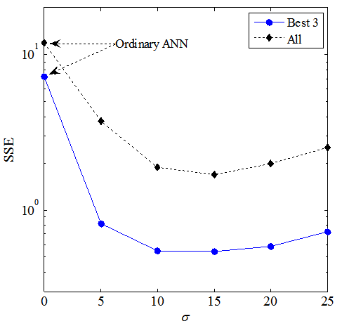 | Figure 8. Average SSEs at each value of σ on the two-nested spirals problem |
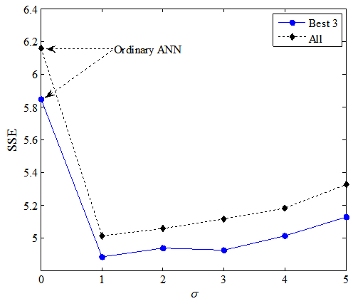 | Figure 9. Average SSEs at each value of σ on the building problem |
5.2. Generalization Ability
In the simulations above, we confirmed that the proposed model has better representation ability by choosing a proper value of σ. However, we need not yet discuss the generalization ability.Figures 10 and 11 respectively show the classification performances of the proposed model withσ = 15 and an ordinary ANN on the two-nested spirals problem. In Figs. 10 and 11, the symbol “o” shows the one spiral  , the symbol “+” shows the other spiral
  , the dotted area shows the area of the spiral of “o” judged by trained proposed model (Fig. 10) and ordinary ANN (Fig. 11), and the white area means the area of spiral of “+”. We used
  for the criterion of the judgment here. It is apparent that the proposed model has better generalization ability than the ordinary ANN on this problem.
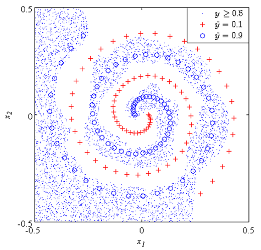 | Figure 10. Classification performance of the proposed model (σ = 15) |
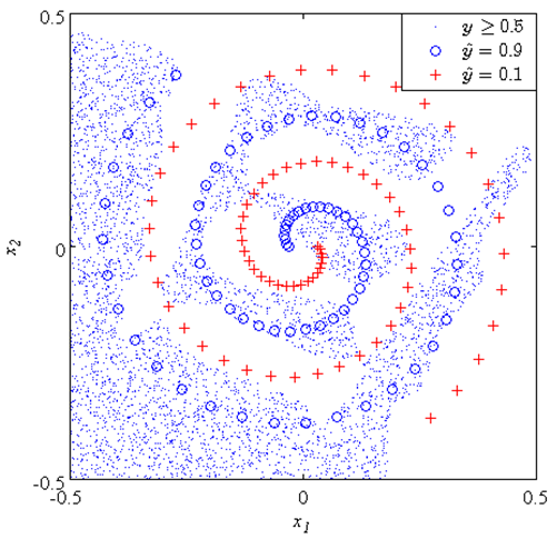 | Figure 11. Classification performance of an ordinary ANN |
In addition, we have given the test set in the dataset building1 to the proposed model that has been trained for the building problem in section 5.2. The test set consists of 1052 examples. Figure 12 presents results of averaged SSE on the best three runs out of the 50 runs and all runs on the test set. In Fig. 12, the superiority of the proposed model for the test set was not observed. Future research will examine how to improve the generalization ability of the proposed model.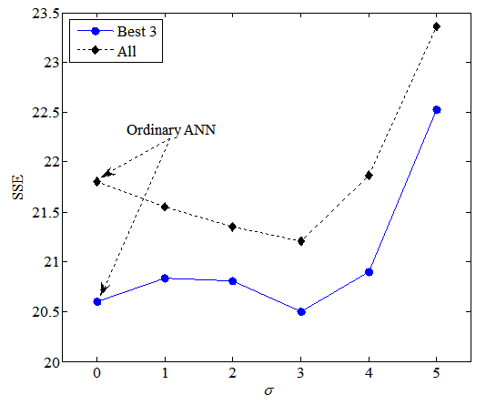 | Figure 12. Average SSEs at each value of σ on the test set of the building problem |
6. Conclusions
This paper proposed a neural network model to control the output of hidden nodes according to input patterns. Based on some knowledge about how the human brain functions, the proposed model has a structure in which an input pattern and a specific node correspond, as well as learning ability. Similar to the cerebellum and the cerebral cortex in the brain the proposed model consists of two parts: The main part with supervised learning, and the SOM control part with unsupervised learning. The structure and the learning algorithm have been discussed. As results of simulation studies showed, the proposed model has better representation ability than that of an ordinary ANN, which shows that controlling the firing strength of hidden nodes according to input patterns improves the efficiency of individual nodes.The parameter σ that controls the firing strength of hidden nodes of the main part is an important parameter for constructing the proposed model. Ascertaining an optimal value of σ remains an open problem that demands further research.
References
| [1] | D. O. Hebb, The organization of behavior – A neuropsychological theory, John Wiley & Son, New York, 1949. |
| [2] | T. Sawaguchi, Brain structure of intelligence and evolution, Kaimeisha, Tokyo, 1989. |
| [3] | A. P. Georgopoulos, A. B. Schwartz, R. E. Kettner, Neuronal population coding of movement direction, Science 233: 1416-1419, 1986. |
| [4] | K. Doya, What are the computations of the cerebellum, the basal ganglia, and the cerebral cortex, Neural Networks, vol. 12, pp. 961-974, 1999. |
| [5] | T. Kohonen, Self-organizing maps, 3rd ed., Springer, Heidelberg, 2000. |
| [6] | Prechelt, L., Proben1-a set of benchmarks and benchmarking rules for neural network training algorithms, Technical Report 21/94, Fakultat fur Informatik, University Karlsruhe, 1994. |
| [7] | D. Whitley and N. Karunanithi, Generalization in feedforward neural networks, In Proc. the IEEE International Joint Conference on Neural Networks (Seattle), pp.77-82, 1991. |
| [8] | Hagan, M. T, H. B. Demuth and M. H. Beale, Neural network design, Boston, MA: PWS Publishing, 1996. |
| [9] | H. Demuth and M. H. Beale, Neural network toolbox: for use with MATLAB, The Math Works Inc., 2000. |
 Abstract
 Reference
 Full-Text PDF
 Full-text HTML