-
Paper Information
- Paper Submission
-
Journal Information
- About This Journal
- Editorial Board
- Current Issue
- Archive
- Author Guidelines
- Contact Us
American Journal of Intelligent Systems
p-ISSN: 2165-8978 e-ISSN: 2165-8994
2014; 4(5): 159-195
doi:10.5923/j.ajis.20140405.01
SHARP (Systolic Hebb - Agnostic Resonance - Perceptron): A Bio-Inspired Spiking Neural Network Model that can be simulated Very Efficiently on Von Neumann Architectures
 Abstract
 Reference
 Full-Text PDF
 Full-text HTML
Luca Marchese
Genova, Italy
Correspondence to: Luca Marchese, Genova, Italy.
| Email: |  |
Copyright © 2014 Scientific & Academic Publishing. All Rights Reserved.
This paper describes a bio-inspired spiking neural network that is proposed as a model of a cortical area network and is tailored to be the brick of a modular framework for building self-organizing neurocognitive networks. This study originated in engineering research on the development of a cortical processor that is efficiently implementable with common digital devices. Thus, the model is presented as a hypothetical candidate for emulating a cortical area network of the cerebral cortex in the human brain. The neuron models are biologically inspired but not biologically plausible.
Keywords: Sparse Distributed Representation, Local Cortical Area Network, Cortical Minicolumn, Cortical Macrocolumn, ALs, Hebb, Winner Takes All, Pattern Recognition, Insect Olfactory System, Spiking Neuron, Rank Order Coding, Agnostic Resonance, Restricted Coulomb Energy, Radial Basis Function, Deep Learning, Probabilistic Neural Network, Evidence Accumulation, Pulsed Neural Network, STDP, Cognitive Systems, Autonomous Machine Learning, Global Workspace, Concept Cells, Neurocognitive Networks
Cite this paper: Luca Marchese, SHARP (Systolic Hebb - Agnostic Resonance - Perceptron): A Bio-Inspired Spiking Neural Network Model that can be simulated Very Efficiently on Von Neumann Architectures, American Journal of Intelligent Systems, Vol. 4 No. 5, 2014, pp. 159-195. doi: 10.5923/j.ajis.20140405.01.
Article Outline
1. Introduction
- In this paper, we propose a spiking neural network model that is inspired by the Drosophila olfactory system and that has both supervised and unsupervised learning capabilities. The philosophy of this research is that everything in the model should be biologically inspired but not necessarily biologically plausible on the basis of current knowledge of the human brain. In the first part of the paper, we analyze the architecture of the network and the behaviors of the neuron typologies that are involved. In the same section, we explain in detail the learning algorithm and some important characteristics of the network.This study originated in engineering research on the development of a cortical processor that is efficiently implementable with common digital devices. Thus, the model is presented as a hypothetical candidate for emulating a cortical area network of the cerebral cortex in the human brain.The second part of the paper analyzes the proposed model as an element of more complex systems. Furthermore, the network is analyzed as a brick of a modular framework for building neurocognitive networks.The third part of the paper is dedicated to the software simulation and the tests. An optimized software simulation demonstrates how this model is very efficiently implemented on Von Neumann computers. In this context, a simulation of the model is analyzed on the XOR problem. Some tests using artificial databases are explained. Then, we make an analysis of the algorithm efficiency on Von Newman computers with considerations about trends in current technology. Finally, there is a brief description of a proposal for the development of a cortical processor that utilizes low-cost commercial digital devices.
1.1. Drosophila Olfactory System
- Insects provide a reference point for the study of basic cognitive processes because they have much simpler brains with respect to higher animals but have extremely efficient and adaptive capabilities for reacting and making decisions in the face of complex environmental situations. The enhanced tools that are currently available in insect neurophysiology have made it possible to explore neural signal processing in specific parts of the insect brain. The insect brain areas that are responsible for complex behaviors, such as attention, are the Mushroom Bodies (MBs) and the Lateral Horns (LHs), which constitute principally the olfactory learning system (Fig.1).
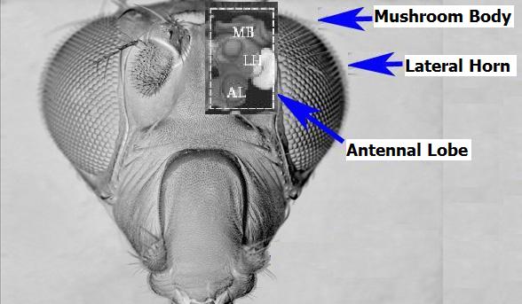 | Figure 1. Simulated X-ray view of the Mushroom Body, Lateral Horn and Antennal Lobe, which are parts of the Drosophila olfactory system |
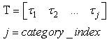
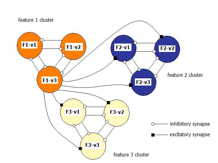 | Figure 2. Simplified interconnection scheme of neurons in the Drosophila olfactory system |
1.2. Agnostic Resonance
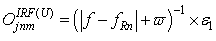
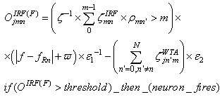
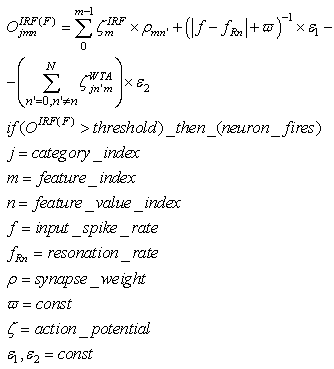
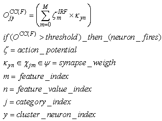
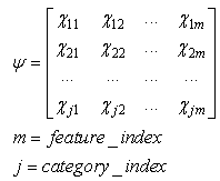
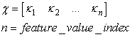
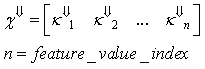
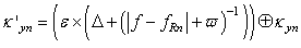
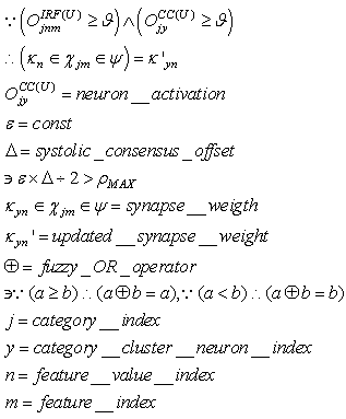
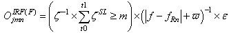
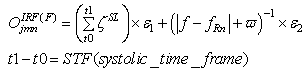
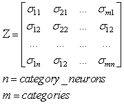
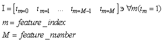
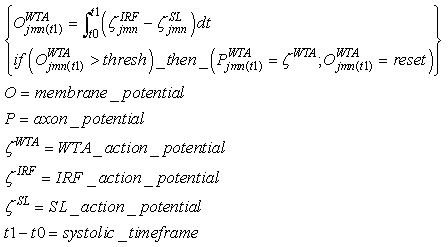
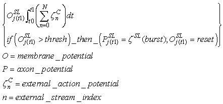
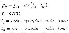
- The first part of the acronym “SHARP” stands for “SystolicHebb” and refers to the learning rule applied to synapses on resonating neurons in a sequential flow. The second part stands for “Agnostic Resonance Perceptron” and refers to the perceptron-like multilayer architecture, where the capability of the neurons in each layer to resonate to a specific value of a feature is “agnostic” because it is not related to previously learned patterns. We have only to remember the meaning of the word “agnostic”.Thomas Henry Huxley, an English biologist, coined the word “agnostic” in 1860.Agnosticism can be defined in various ways and is sometimes used to indicate doubt or a skeptical approach to questions. Since Huxley coined the term, many other thinkers have written extensively about agnosticism, and its meaning now has many nuances that are related to religion and philosophy.We are interested only in the etymology of the word from ancient Greek: Agnostic (Greek: ἀ- a-, without + γνῶσιςgnōsis, knowledge). Then, we define “agnostic resonance” as a resonance that is not generated by knowledge. In the ART (Adaptive Resonance Theory) paradigm, a neuron resonates in response to an input pattern that is similar to its prototype. In our model, this type of knowledge-based resonance does not exist at the level of the neuron but only at the level of the network because the neurons are related to a specific value in a specific feature. In this context, we can speak about “agnostic resonance” because the neurons do not resonate according to the whole pattern (knowledge) but only to a fixed value of a single feature.The network can be viewed as an ensemble of clusters or in a more classical fashion as a multilayer network in which any layer is related to a single feature. Stimuli are connected directly to each layer.Any neuron of any layer is connected to any neuron in the subsequent layers with a weighted synapse. Any neuron in any layer is connected to the category layer through weighted synapses.The category layer is organized in the WTA mode (Fig.4). In this architecture, the features have been “ordered” in such a way that the neurons that are related to feature f(n) send spikes to the neurons that are related to the features f(n+1), f(n+2), …, up to f(m) (m is the maximum number of features), while the feature f(m) does not send back spikes to the feature f(m-1), and so on. Feed-forward spikes work as “enabling” signals for the subsequent feature neurons. We have defined this behavior as “systolic”, which refers to blood flow: this term has been used in past years to define a class of parallel computers in which all of the processors were connected in a sequential chain: systolic systems for computer calculus were defined by professor H.T Kung(Carnegie-Mellon University) in his paper “Why Systolic Architectures?” [32]. A neuron that is associated with the feature f(n) must receive a spike from one neuron in the n-1 previous feature layers to be “enabled” to fire. If a neuron is “enabled” and it is resonating with the input value, it fires, sending a spike to the subsequent layers. The systolic flow and the agnostic behaviors are strictly correlated with the time domain, and the feed-forward spikes in such an architecture carry “evidence accumulation”.In this network, we define a type of neuron that we have called “Integrate, Resonate and Fire” (IRF). This neuron reaches an enabling threshold, integrating spikes that come from resonating neurons in the previous features. Any layer that is associated with a feature is organized into a WTA modality. The network can be realized with another type of Integrate and Fire (IF) neuron that is composed of two integration sections, which work in Rank Order Coding for the feature input signal and in flat integration for the enabling spike inputs. We have called this neuron Hybrid Integrate and Fire (HIF). The only difference between the two types of neuron is the input decoding modality.The category neurons are connected to each neuron in each feature layer. We use two different activation functions for the learning activity (synapse update) and for the recognition activity (firing neuron) because the synapse update is proportional to the only resonation level.The feature neurons are defined as follows:1) IRF (Integrate - Resonate - Fire):In this neuron model, the input value is represented by the frequency of the spikes, and any neuron that is associated with a specified feature is resonating at a specific frequency. Due to the undesired resonation of the neurons with near resonating frequency values, all of the neurons that are associated with the same feature are connected among themselves through inhibitory synapses, to obtain a WTA behavior. Any neuron must be triggered by a sequence of spikes that originates from the back-layers, to emit a spike.SUA (Synapses Update Activation):
 | (1) |
 | (2) |
 | (3) |
 | (4) |
 | (5) |
 | (6) |
 | (7) |
 | (8) |
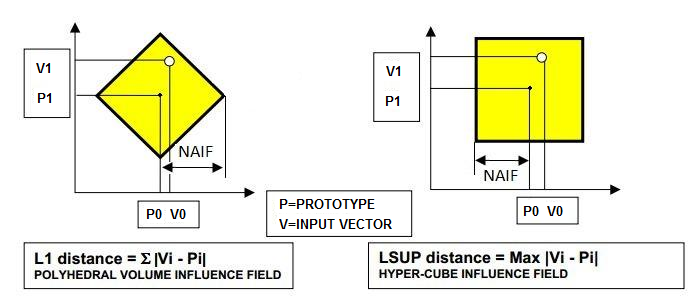 | Figure 3. The mathematical concepts of the L1 distance and LSUP distance |
 | (9) |
 | (10) |
 | Figure 4. Category neurons are connected among themselves with inhibitory synapses in the same way as neurons inside feature clusters. These inhibitory connections ensure a WTA behavior in the category layer |
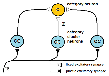 | Figure 5. Category cluster neurons work in a daisy chain that is tailored to manage a handover of learning activity, to limit the number of patterns that are learned by a single neuron and thus limit the crosstalk effect |
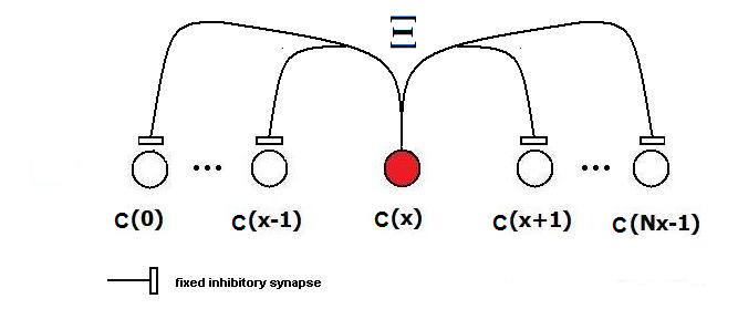
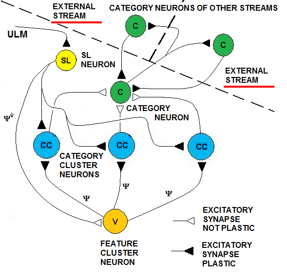
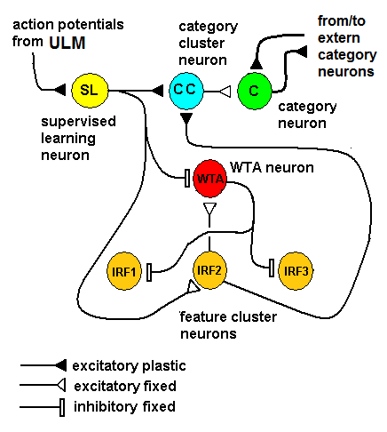 | Figure 6. Inside a cluster that is associated with a feature, neurons (that are associated with specific values of such a feature) are fully interconnected through inhibitory neurons (WTA neuron) that are in turn inhibited by the action potential from the category neurons. This mechanism disables the WTA when the category neuron is activated by external action potentials (supervised learning), permitting the nearest neighborhood neurons to fire and STDP to be applied to their synapses. This behavior makes the network able to generalize |
2. UNLEASH: Unified Learning by Evidence Accumulation through Systolic Hebb
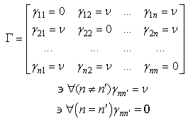
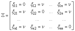
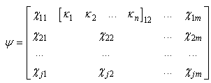
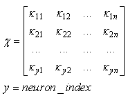
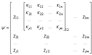
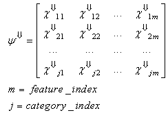
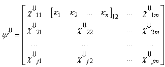
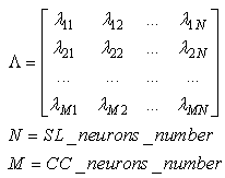
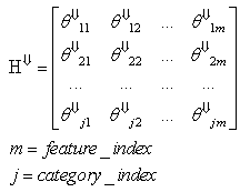
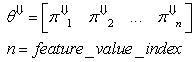
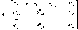
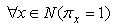
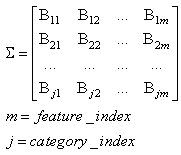
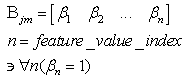
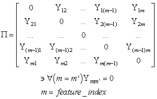
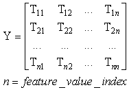
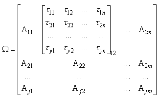
- The learning algorithm that is presented in this paper updates the synapses among the IRF neurons that are associated with specific values of different features when these neurons resonate. The synapses are updated with direct proportionality to the resonation level.The synapse that connects the resonating neurons with the active category neuron is updated by following the same rule. The learning steps are as follows:1. In any feature layer, the input frequency makes one neuron maximally resonating and activating. Nearest neighborhood neurons in the same layer resonate and activate also, with a strength that decreases by the distance. 2. The synapses between the spiking neurons in the feature cluster ‘n’ and all of the spiking neurons in the following feature clusters (n’ > n) are updated following the STDP rule. These synapses assume a value that is proportional to the minimum level of resonance between the connected neurons.3. The synapses between the spiking neurons in the feature clusters and the spiking neuron in the category cluster (activated by action potentials from the SL neuron as in Fig.6) are updated. They assume a value that is proportional to the resonance with the input signal. If the active neuron in the category cluster reaches a number of active afferent synapses that is greater than a specific threshold, it loses the capability to learn and hands over this capability to the next neuron in the cluster chain. To define mathematically the behaviors that are described in the above steps, we must define mathematically the synaptic structure of the network. The matrix of lateral inhibitory connections between IRF neurons is obtained through a WTA neuron that is associated with any IRF neuron (Fig.6):
 | (11) |
 | (12) |
 | (13) |
 | (14) |
 | (15) |
 | (16) |
 | (17) |
 | (18) |
 | (19) |
 | (20) |
 | (21) |
 | (22) |
 | (23) |
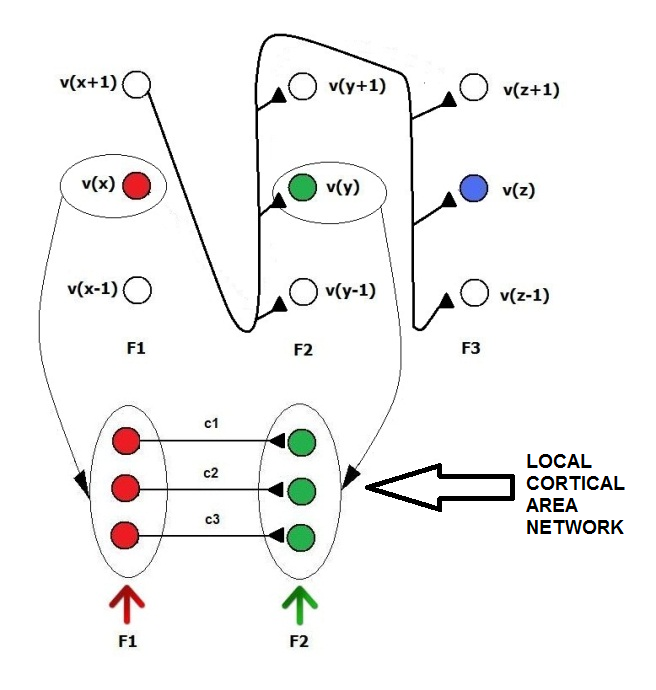
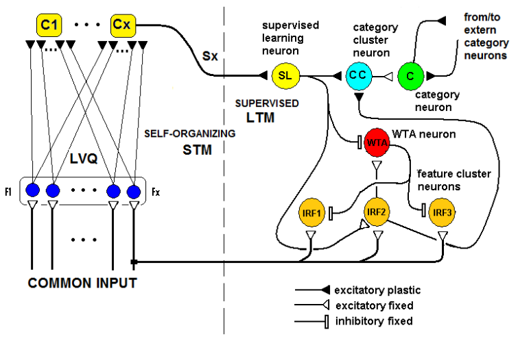
 | Figure 7. Functional view of the SHARP network. In the lowest side, the clusters that are related to features (F1, F2, F3) are shown, and their forward excitatory interconnections form any F |
 | (24) |
 | (25) |
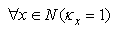
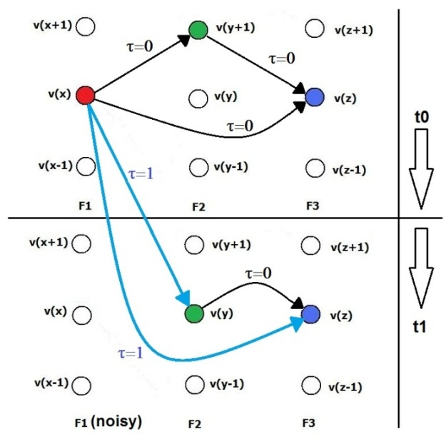
 | Figure 8a. The excitatory synapses activated from the first layer to the subsequent layers. In the considered case, a pattern that is composed of F1=v(x), F2=v(y) and F3=v(z) is learned. The neurons v(x-1), v(x+1), v(y-1), v(y+1), v(z-1) and v(z+1) are the neighborhood neurons of the primary resonating neuron. They are responsible for the generalization capability of the neural network. The size of the neighborhood area is dependent on the activation (SFA) formula and the firing threshold. In the picture, we have considered a neighborhood of size 1 for simplicity of representation. The activity of the neighborhood is disabled by the intra-cluster inhibitory activity, which is in turn disabled by the inhibitory activity from category neurons for a while when they are activated by action potentials from external activities (supervised learning). At the top of the picture, there is a reference to the possible mapping of the proposed architecture to the cortical hyper-column and mini-column |
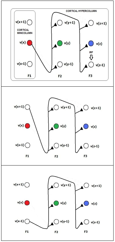
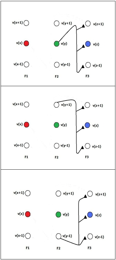 | Figure 8b. The excitatory synapses, activated from the second layer to the subsequent layer. In the considered case, a pattern that is composed of F1=v(x), F2=v(y) and F3=v(z) is learned. The neurons v(x-1), v(x+1), v(y-1), v(y+1), v(z-1) and v(z+1) are the neighborhood neurons of the primary resonating neuron. They are responsible for the generalization capability of the neural network. The size of the neighborhood area is dependent on the activation (SFA) formula and the firing threshold. In the picture, we have considered a neighborhood of size 1 for simplicity of representation. The activity of the neighborhood is disabled by the intra-cluster inhibitory activity, which is in turn disabled by the inhibitory activity from the category neurons for a while when they are activated by action potentials from external activities (supervised learning) |
 | Figure 9. Any neuron in any cluster that is related to a single feature has a clone for any category. The input synapses are replicated, while the axons that are associated with different categories are independent. This ensemble of clone modules should represent a cortical area network |
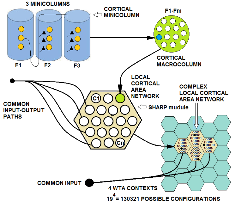
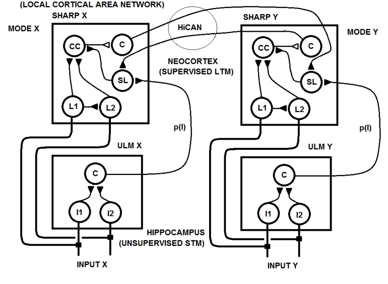
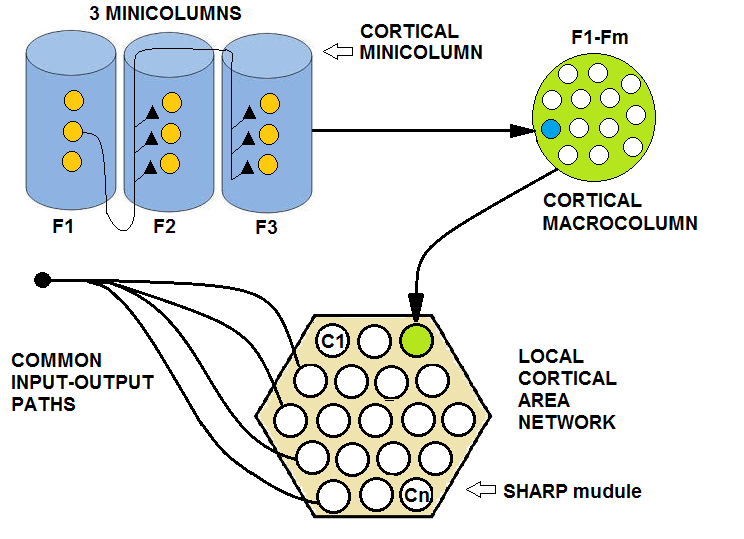 | Figure 10. The dense short-range interconnection of a set of macrocolumns in a local area of the cerebral cortex, together with common input and output pathways, constitutes a local cortical area network. A SHARP module should represent a local cortical area network. Any feature cluster is a minicolumn, and the ensemble of all of the feature clusters is a macrocolumn. A macrocolumn identifies a part of a distributed representation of a category or the category itself in the higher level of the hierarchy |
 | (26) |
 | (27) |
 | (28) |
 | (29) |
 | (30) |
 | (31) |
 | (32) |
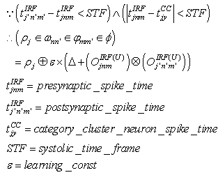
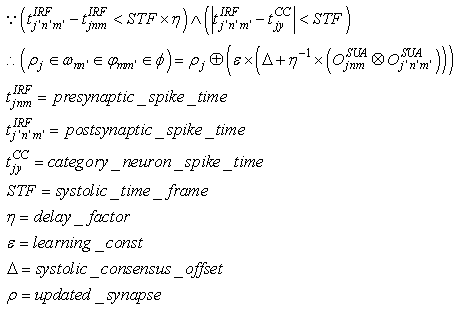
 (excitatory fixed)enable supervised learning. They transport the spikes from the SL neuron, which are activated by spikes that are generated outside of the network, to neurons in the feature clusters that are associated with the category, enabling them to fire and disabling the WTA behavior. The synapses between resonating neurons in different clusters can be updated because these neurons fire as a result of the contribution of action potentials from the SL. When these synapses become sufficiently conductive, unsupervised reinforcement learning through STDP can occur without the contribution of the SL neuron (Unified Learning). Spike timing in the systolic structure of the clusters reflects the sequence of the features. The spike of the category neuron could occur before or after the spike of the postsynaptic IRF neuron but within a range that is limited by the STF (Systolic Time Frame).STF is the total time that is required for the complete propagation of spikes through all of the feature clusters.Thus, (29) is reformulated as follows:
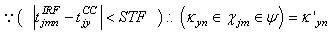 | (33) |
 | (34) |
 | (35) |

 | (36) |
 | (37) |
 | (38) |
 | (39) |
 | (40) |
2.1. Neural Phase-Locked-Loop Circuit
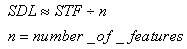
- There is an important issue that is related to the behavior of the neural network that is presented in this paper. In the definition of the learning algorithm that is based on STDP, we have used the STF parameter as the time that is required to complete a full sequence of spikes through the feature clusters. We have also defined the SDL as the basic time that is required for a spike to pass through a cluster-to-cluster synapse. The SDL is roughly a fraction of STF:
 The IF neurons that are used in SHARP do not leak membrane potential as in the more biologically plausible LIF (Leaky Integrate and Fire) model and must be reset at the right time if the neuron is not firing. In the next chapter, a detailed explanation of the neuron models will clarify this concept. The reset of the neurons that remain in a transition state is warranted by a PLL (Phase Locked Loop) circuit that locks on the phase of the action potentials from the neurons of the first feature cluster.The neural PLL circuit is composed of a chain of neurons, which reflects the systolic sequence of the feature clusters. The last neuron in the chain produces an inhibitory activity on all of the neurons in the network.This retroaction makes the neural network working as an oscillator with the STF as a period. In this framework, we define local cortical area networks as neural oscillators that behave asynchronously within their own network.The synapses in the NPLL circuit are excitatory and inhibitory but fixed. The learning process does not affect at all the behavior of the circuit (Figs.11 and 12). Next, we must define the matrix of synapses that are involved in the NPLL circuit.
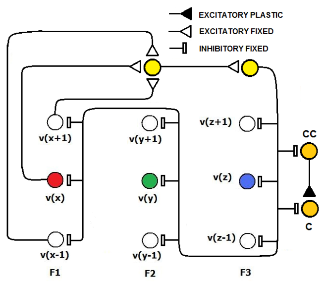 | Figure 11. The N-PLL circuit inhibitory activity is triggered by the action potentials that are emitted by the IRF neurons in the first feature cluster. The neurons are IF neurons that have a threshold that can be exceeded with a single spike. Any synapse between PLL neurons adds an SDL delay to the propagation of the signal |
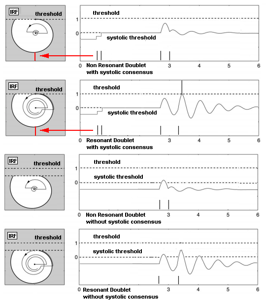
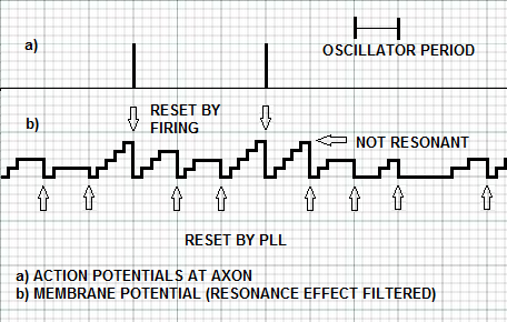 | Figure 12. The membrane potential of an IRF neuron that is filtered from the effect of resonance with the input stimulus. A complete firing consensus is reached three times, but only two of those times are synchronized with resonance. When the neuron fires, the membrane potential is automatically reset. When the neuron does not fire, the inhibitory spike from the N-PLL neurons provides the reset of the membrane potential |
 | (41) |
 | (42) |
 | (43) |
3. Neuron Models
- There are five types of neurons that are involved in the SHARP model:1. IRF (in the feature clusters)2. WTA (in the feature clusters)3. C (the category neurons)4. SL (supervised learning)5. CC (in the category clusters)In this part of the paper, there is a detailed description of the behavior of any neuron type that is involved in the presented neural network.
3.1. IRF (Integrator-Resonator)
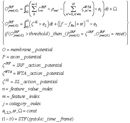
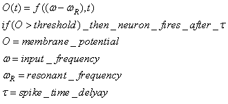
- This neuron model is a combination of the integrate-and-fire model and the resonate-and-fire model. In the IRF neuron, the firing threshold can be reached only through the integration of spikes from different dendrites combined with the resonation of a pair of spikes, often referred to as a “doublet”, on a single dendrite. The resonating part of the neuron behaves in such a way that each pulse alone cannot evoke an action potential, but a pair of spikes can, provided that they have appropriate timing [5][6]. In a classical resonate-and-fire neuron, the appropriate timing of such a doublet can push the internal potential beyond the threshold. In the IRF, the second pulse can do the same only if the internal potential has already reached a certain value due to the integration of the spikes that come from other dendrites. If the neuron reaches the required “offset” of the potential, it can exceed the firing threshold only if the inter-spike interval of the doublet is infinitesimal or if such an interval is equal or very near the eigenperiod that is typical of the neuron [5]. The eigenperiod that is typical of the IRF neuron is strictly correlated with the discrete “feature value” that is associated with the neuron.
 | (44) |
 | Figure 13. IRF neuron behavior is driven by the systolic spikes that come from previous feature clusters and by the spikes whose temporal interval represents the value of the feature. The picture shows the four possible cases, of which only one can generate an action potential. This example refers to the third feature cluster in the systolic chain (two systolic spikes). The interval between the spikes has been relaxed to make a clearer picture |
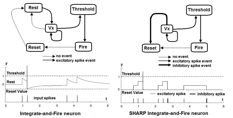 | Figure 14. On the left, the more biologically plausible Integrate and Fire neuron behavior. On the right, the simplified Integrate and Fire neuron that is used in SHARP. In the states machine, Vx represents any value that is between Rest/Reset and Threshold |
3.2. WTA (Integrator)
- This neuron performs the WTA behavior in the feature clusters, and there is one WTA neuron for any IRF neuron. They provide the WTA behavior only when there is not supervised learning. A WTA neuron is excited by the associated IRF neuron, and it is depressed by the activity of the SL neuron in the same category; it works like an integrate-and-fire neuron, but the SL signal is inhibitory.
 | (45) |
3.3. C (Integrator)
- This type of neuron is a classical integrator. Category neurons are activated by the whole sequence of spikes from feature clusters or by the spike train from an SL neuron during supervised learning. In both cases, the spikes pass through the CC neuron that is currently active. The threshold is set in such a way that the membrane potential can reach such a value only when the neuron receives a spike from any feature cluster. If the SL neuron is firing, then the membrane potential can reach the threshold as a result of this contribution. There is an inhibitory activity of all of the other Category neurons that ensures the WTA behavior.
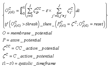 | (46) |
3.4. SL (Integrator)
- Supervised Learning neurons receive action potentials from external streams, which provide a supervised learning activity. They send action potential sequences to the IRF neurons in the feature clusters that are associated with the same category. These action potentials replace the spikes that arrive from the back-clusters and enable the resonating neurons to fire, making STDP applicable. SL neurons activate the C neuron, enabling it to fire and making STDP applicable also between IRF resonating neurons and the active CC neuron. The SL neurons deactivate the WTA neurons. In this way, the neighborhood IRF neurons fire, and STDP can be applied, which enables us to obtain the LSUP distance generalization.The action potentials that are generated by the SL neurons are in the form of bursts. The bursts replace the single spikes that come from the IRF neurons. Thus, the number of spikes in the burst is related to the feature cluster.
 | (47) |
3.5. CC (Weighted-Selective-Integrator)
- Category Cluster neurons limit the crosstalk between new and old learned patterns. These neurons have plastic synapses that are connected with axons of IRF neurons. They “share” learning activity with the other CC neurons in the same cluster. CC neurons work in a “daisy chain”: when neuron n reaches the threshold of the activated synapses, it loses the capability to learn and transfers this capability to neuron n+1, and so on.This neuron has dendrites that are connected to all of the IRF neurons in any feature cluster but has a characteristic threshold of “maximum density” of the activated synapses.It is possible to see in the formula that the contribution of the spikes from the IRF neurons is weighted. The characteristic behavior of this neuron is concentrated in the role of synapse
 which enables or disables the influence of the SL neuron depending on the amount of past plastic activity of the synapses. If the density of the activated synapses (k>0) exceeds the threshold, then the action potential from the SL neuron cannot trigger learning. Here,
  is the excitatory synapse between the SL neuron and the CC neuron, and its plastic activity is almost on-off; it is driven by an integrative process of the plastic activity of the synapses that are connected to the IRF neurons.
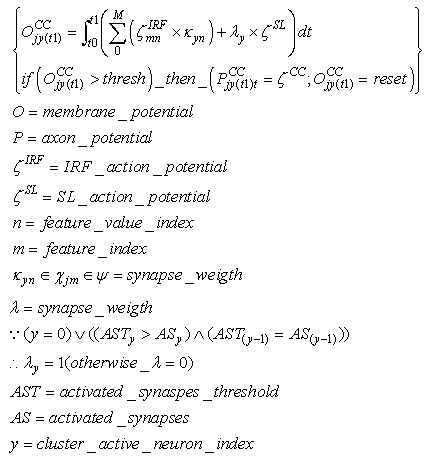 | (48) |
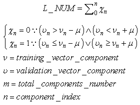
4. Pattern Recognition: Generalization through LSUP and LNUM
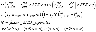
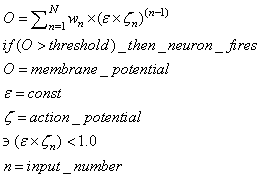
- The behavior of the network, when no category neuron is activated by an external signal, is a pattern recognition activity.When a pattern is received as input, one neuron in any layer resonates and activates. In this phase, a neuron reaches a full activation state only if it has received a spike from a single neuron in any previous layer. Spikes from previous layers arrive to a resonating neuron if the synapses between the resonating neurons in any layer have been activated in the learning phase. This circumstance means that the input pattern or a similar pattern (inside the maximum LSUP distance) has been previously learned. The recognition is positive if any resonating neuron receives an “enabling” signal (a spike) from any previous layer and if at least one category neuron has conductive synapses with all of the activating neurons. The recognition strength can be evaluated in two different ways:• the first way is to evaluate the minimal synapse strength with a fuzzy-AND operator• the second way is to evaluate the average of the synapse strengthsMore than one category neuron can be excited. WTA connections in the category layer guarantee that only one category neuron can be activated.Computation of the recognition strength with the fuzzy-AND operator:
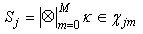 | (49) |
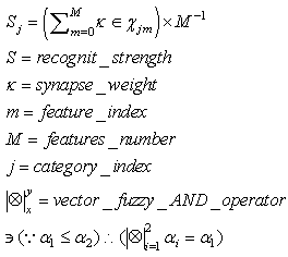 | (50) |
5. Plasticity Driven by Class Specialization
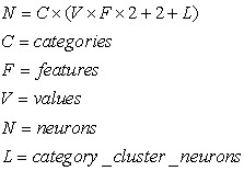
- The number of inputs or features is entirely managed by the category nodes, and a new category node that is connected only to a subset of feature clusters can be added. This new category node must have a congruently limited activation threshold. In the same way, new feature clusters and related category nodes can be added. SHARP can grow in the number of features, and new category nodes represent concepts that are specializations of existing categories.The fundamental aspect of this behavior is that plasticity is realized in three ways:• Synapse updating• New category nodes• New featuresThe third modality is the “plasticity by class specialization” that is shown in Fig.15. This type of plasticity, which is performed with the creation of new neurons, could be triggered in the brain by detecting the crosstalk effect between learned patterns. Such a behavior would be the equivalent of the mismatch condition in the Adaptive Resonance Theory, but the probability of mismatch is forecasted on the grounds of measured crosstalk. This mechanism must be enabled by another process that is capable of detecting the availability of additional discriminant features. We are currently working on the algorithms that could implement these two behaviors.
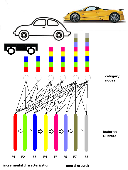 | Figure 15. A very simplified example of PCS. The example does not account for the fact that the concept is in reality built by the cooperation and/or hierarchy of multiple streams |
6. Do Spikes add Entropy in this Architecture? With which Coding Scheme?
- SHARP is an NN whose neurons communicate through spikes. We have analyzed neuron models that can manage appropriately spikes that are received at their dendrites, computing the possibility to fire a spike on their axon. We have built such a framework while moved by the desire to mimic biological brain behavior. Can we say that this neural network is a third generation model? To answer this question, we must clarify some concepts.We normally classify second generation neural networks as those neural paradigms that use analog values to encode information. Neural networks of the third generation use spikes to encode the information that is transmitted between the neurons. Any neural network of the second generation can be transformed from a spiking model by representing analog values for the firing rates of the spikes. Thus, we generally refer to the third generation only for those NNs where the timing of a single spike is meaningful.A number of studies have investigated the computational efficiency of the NN based on the spiking neurons. Maass demonstrated that a NN that is based on spiking neurons holds more computational power than a NN of the first and second generation. Spiking NNs have been identified as universal approximators because they can simulate NNs of the second generation [7], which are universal approximators themselves. In fact, Maass formulated and demonstrated these theorems using a precise definition of spiking neural networks [8]:• A finite set V of spiking neurons.• A set V_in and a set V_out of input and output neurons.• A set of synapses that cannot be incoming to input neurons• A weight w for each synapse• A response function
 • A threshold function
  • A delay
  for each synapseIn spiking NNs, the rate-versus-timing debate has been framed as a question of whether all of the information about the stimulus is carried by the firing rate (or by the spike count in some specified time window) or whether the timing of individual spikes within this window also correlates with the variations in the stimulus [9]. This debate cannot have a single answer because spikes can play different roles in different contexts and thus they can encode information in multiple appropriate manners.The basic consideration is that spikes are, probably, the most appropriate method for transmitting information within biological matter, and we use the term “appropriate” while referring to physical issues and not to information theory. From the point of view of information theory, Maass demonstrated that the spiking neural code can carry more entropy.Entropy, as defined in thermodynamics and statistical mechanics, is a measure of “variability” or “available information”.We can define, mathematically, entropy as the logarithm of the number of possible states that the system can assume:
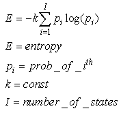 | (51) |
 | (52) |
 | (53) |
 | (54) |
 | (55) |
 | (56) |
 | (57) |
 | (58) |
 | (59) |
 | (60) |
 | (61) |
 | Figure 16. The LTIM generalization capability of SHARP. At the instant t1, the feature F1 is extremely noisy and, assuming that LSUP is set to 0 or saturated, the history of the feature relationships enables the recognition of the pattern as a result of spikes that are transmitted through delayed synapses |
7. Autonomous Machine Learning
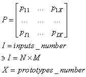
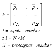
- The learning activity of SHARP is triggered by a spike train to an SL neuron from an external module. In a neurocognitive network, modules that are associated with different modalities should be able to learn autonomously and thereby start a cooperative process. A method for deciding whether the current stimulus must be learned and associated with some “unlabeled” category node is using a probabilistic method. The network should trigger a learning activity when the same stimulus has been received more frequently than others in a relatively large timeframe.We have provided unsupervised learning by adding an external modulethat associatesun supervised learning with STM (Short Term Memory) and supervised learning with LTM (Long Term Memory). The module is a spiking Learning Vector Quantization (LVQ) neural network. Any prototype is connected to an “unlabeled” category neuron and is continuously updated by the input patterns. We have called this module ULM (Unsupervised Learning Module).ULM works as a “working memory” in which the input patterns are memorized for a short period of time. For a frequent input pattern, the LVQ process moves the synapse weights of the nearest prototype in the direction of the pattern. When the input pattern is very close to the prototype, the associated neuron is excited over the threshold and emits a spike.Fig.17 shows the connections between ULM and SHARP.
 | Figure 17. The connection scheme of the “Unsupervised Learning Module” together with the SHARP module. P1, P2, P3 are the prototypes of the ULM that constitute the Short Term Memory. For simplicity, ULM has only three prototypes, and SHARP is shown partially (only the feature Fx-1 cluster with three value neurons IRF1, IRF2, IRF3). Neurons in the prototypes of ULM are connected to the category neurons of ULM with plastic synapses (s1, s2, s3). The strengths of s1, s2 and s3 decay over time but grow when the prototype is resonating with an input pattern. The most important part of this scheme is the sC3 synapse that connects the ULM with the SHARP module. This synapse is plastic and decays when crossed by action potentials |
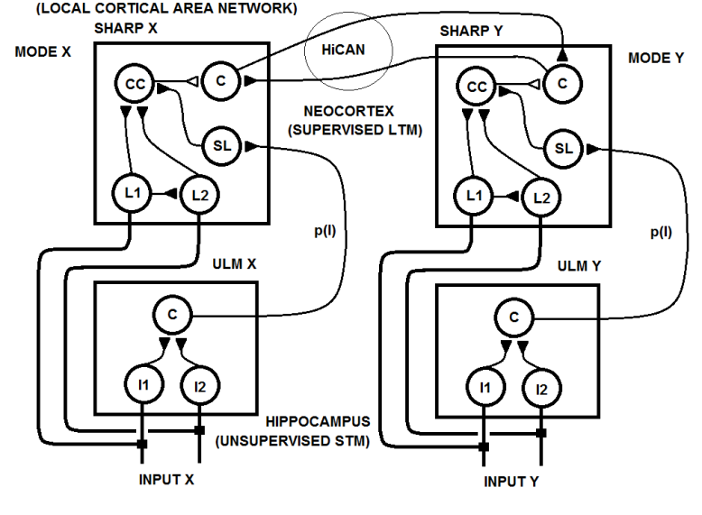
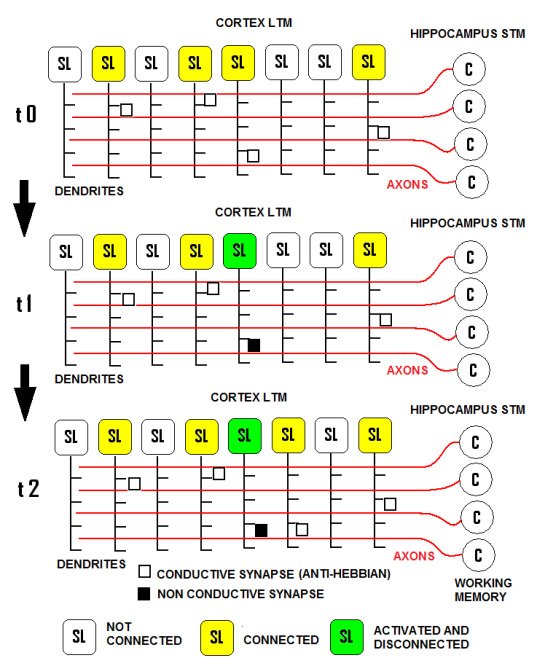 | Figure 18. The interconnection matrix between our model of STM or working memory (the ULM module), which works in an unsupervised manner, and our model of LTM (the SHARP module), which waits for an external teaching signal on the SL neurons to activate a category node. Any SL neuron can be connected with only one axon from the working memory, and vice versa. When a neuron of the ULM (C) emits action potentials, the SL neuron that is associated is activated, and the anti-Hebbian synapse is deactivated. This SL neuron loses the possibility of receiving other inputs from the ULM |
 | (62) |
 | (63) |
 | (64) |
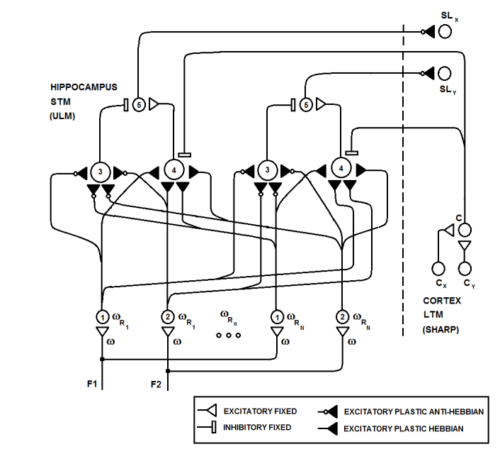 | Figure 19. Details of the neural circuit in the ULM with two features (F1, F2) and N resonation values in the input grid (neuron types 1, 2). Neurons of types 3 and 4 are Rank Order Integrate and Fire with anti-Hebbian and Hebbian synapses, respectively. Neurons of type 5 fire when the excitatory activity of neurons of type 4 exceeds the inhibitory activity of neurons of type 3. This circumstance occurs when the same pattern is presented very frequently and, thus, a training signal is sent to the cortex (SL neurons). Category neurons in the cortex inhibit neurons of type 4, and thus, a pattern that is recognized at the LTM level cannot be learned at the STM level |
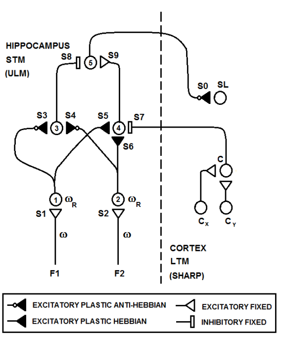 | Figure 20. A simplified view of the circuit shown in Figure 19. Only the neurons that are related to one resonation value are shown. It can be seen that there is a pair of neurons (3, 4) for any prototype, and any input neuron connects to any neuron 3 with anti-Hebbian synapses and to any neuron 4 with Hebbian synapses. The circuit would be the same considering one feature and two resonation values. Neuron C in the cortex fires when an input pattern is recognized (one category of neuron fires) |
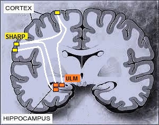 | Figure 21. The hypothetical position in the brain of the SHARP modules (local cortical area networks) and the associated ULM modules. Local cortical area networks should interconnect with one another in the cortex layers or possibly through white matter. Short Term Memory modules in the Hippocampus should connect to local cortical area networks in the cortex through white matter |
 | (65) |
 | (66) |
 | (67) |
 and is given as follows:
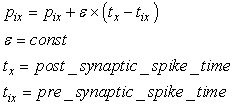 | (68) |
 | (69) |
 | (70) |
 | (71) |
8. Deep Learning in Hierarchy and Composite Complex Structures
- It is universally recognized that the brain is intrinsically parallel but is also a hierarchical structure. Hierarchy is a fundamental concept in any complex behavior; thus, we must explore how the proposed model could work in a hierarchical structure. This exploration is a fundamental analysis for the purpose of measuring how efficiently the elementary behavior can be a “brick” of a more complex system and thus, in our case, of the brain.It is possible to reduce the LSUP maximum distance in the learning activity, thus providing higher specialization of the concepts that are in lower levels of the hierarchy. As an example, “vehicle” would be a parent class of “car” and “truck”.In the SHARP simulation on the computer, the processing speed is independent of the number of examples learned. The number of synapses is, instead, directly proportional to the number of categories that are required for the classification. In a software implementation, the larger the number of classes is, the larger the memory that is required to store the synapses, and the execution time is linearly affected. Thus, building a hierarchy of SHARP modules by clustering categories (or classes) is a way of reducing drastically the memory that is required for the synapses. Hierarchy is not the only way that multiple SHARP networks can be interconnected to produce more complex neural networks and behaviors. For example, multiple SHARP networks can be connected to have the same global input pattern but different identification tokens of the associated category. In this way, the bottleneck of the synapses that are associated with the categories can be easily solved:
 | (72) |
 | Figure 22. Multiple SHARP networks are connected to the same inputs, and learn only a token of the distributed category representations. This configuration can be considered to be a complex cortical area network. A total of 4 modules that are composed of 19 hyper-columns can represent 19^4 configurations |
9. Hierarchical Concepts Associative Nodes in a Self-Organizing Neurocognitive Network
- Multiple parallel streams in the brain communicate among themselves during an information processing flow. These streams are cognition processes or sensorial processes that communicate among themselves at different levels, merging and integrating information through inter-stream channels. We have attempted to analyze how SHARP could be one type of the bricks that are components of a complex neurocognitive network. The approach that we propose in this paper is well known in literature [13] and we only have inserted the SHARP modules in such a framework adapting some concepts to the neural network model. We have defined HiCANs (Hierarchical Concept Associative Nodes), which should behave as channels for inter-stream communication. The principal idea is that HiCAN(s) work as nodes where knowledge of a specific stream can be associated with knowledge of another stream.We have defined a framework in which a neurocognitive network grows around simple learning elements that each process a single stream. We have analyzed here how the proposed neural network can be the basic learning element of the system while not excluding that other different behavioral elements could be included. Category nodes are directly connected to HiCAN(s) because a category node can be activated by another category node of another stream, as shown in Fig.23.
 | Figure 23. Two Concept Associative Nodes. These are inter-stream interconnections between category neurons of different streams |
 | Figure 24a. A multimodal concept network (HiCAN) is created through the STDP between two category neurons in the two cortical area networks |
 | Figure 24b. In the second hypothetical circuit, a multimodal concept network (HiCAN) is created through STDP between the category neurons and the SL neurons in the two cortical area networks |
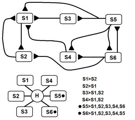 | Figure 24c. In the HiCAN that is shown, s1, s2, s3, s4, s5 and s6 are connected streams. In this HiCAN, only S5 and S6 represent a complex concept. The bottom-left simplification is useful for representing complex networks of interconnected streams, such as in Fig. 24c |
10. Optimized Software Simulation
- In the history of neural networks, pattern recognition problems have been a paramount application target and benchmark.In recent years, we have observed development of many new paradigms more or less inspired by biological systems. These often have been applied to pattern recognition problems running on Von Neumann architecture computers. Due to the serial nature of these computers, many paradigms suffer low performance for real time applications, whereas others do not show capability to store many new patterns without losing or affecting previous knowledge (plasticity versus stability problem). We have proposed a paradigm inspired by the Drosophila olfactory system that can be simulated very efficiently on Von Neumann architectures.Following these concepts, synapses between feature neurons have been simulated with a 4-dimensional matrix of bytes while synapses between feature neurons and category neurons have been simulated with a 3-dimensional matrix of bytes. Below we will analyze the operations performed during the learning phase and during the recognition phase.• In the learning phase, the following conditions are met:Any synapse in the 4-dimensional byte-matrix connecting two resonating neurons is updated.Any synapse in the 4-dimensional byte-matrix connecting a resonating neuron with neighborhood activating neurons in different layers is updated. Any synapse in the 3-dimensional matrix of bytes connecting a resonating neuron or a neighborhood activating neuron with a category neuron is updated. The maximum value is assigned to this synapse in the case of a resonating neuron. In the case of a neighborhood neuron, the value assigned to the synapse is inversely proportional to the distance of the neighborhood neuron from the resonating neuron.• In the recognition phase, the following conditions are met:Any resonating neuron in any layer checks in the 4-dimensional bit-matrix if it has received a spike from resonating neurons in any previous layer. If this condition is not verified, the process is interrupted and the input pattern is not identified. Any resonating neuron that verifies the reception of spikes from the preceding layers activates category neurons, sending spikes on the weighted routes defined in the 3-dimensional byte matrix. This operation can be performed by averaging the value of the synapse (in byte matrix) with the current activation of the category node or by operating a fuzzy-AND between the same elements. Considering the type of operations performed during the learning and recognition phases, it is clear that this algorithm does not require any complex mathematical operators; instead, the algorithm requires only simple read and write operations from and to memory. The number of read and write (r/w) operations is not correlated to the number of patterns the neural network has learned but is fixed. Actually, the number of memory r/w operations is proportional to the number of features. Such software implementation requires poor computation capability and fixed, small or almost null parallelism. This algorithm places a large demand on memory space to memorize the huge number of synapses. From the previous considerations, we can assert that this algorithm is “tuned” with the current commercial technology. Currently, microprocessors use limited parallelism with memory sharing, and they can actually still be classified as Von Neumann machines. Furthermore, in the last twenty years, memories have grown at a much faster rate than processor speed (clock frequency), and the current trend is still the same. We have created three pattern recognition test-benches with different targets. They are based on sets of artificial databases of random patterns generated by a program appositely designed for this test. These artificial tests are necessary to reach the capacity limits of the network, having full control of statistical parameters of the training set.
10.1. XOR Test
- The first theoretical test that we have conducted on the network is the XOR (exclusive OR) test to investigate if the network can solve this problem as a MLP with two hidden layers or as an RBF neural network. This theoretical test is executed to verify the capability of the neural network to perform correctly on problems that are not linearly separable. The typical function used to execute this test is the logic function of exclusive or. As it is well known, the single layer Perceptron cannot learn this function, whereas MLP does. The not linearly separable function of XOR is shown in Fig. 25. SHARP demonstrates its ability to work correctly with the XOR problem. The resulting network is shown in Fig. 27; Fig. 26 represents the related spikes raster. It is important to remark that SHARP, although the last letter of the acronym stands for “Perceptron”, does not have anything in common with the classical Perceptron. Thus, the number of layers is not relevant. Actually the number of layers in SHARP is exactly equal to the number of features of the problem (in the Perceptron, this is the number of inputs in the input layer).
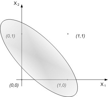 | Figure 25. The representation of the XOR problem |
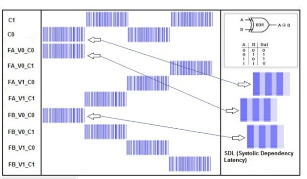 | Figure 26. The spikes raster related to the XOR problem |
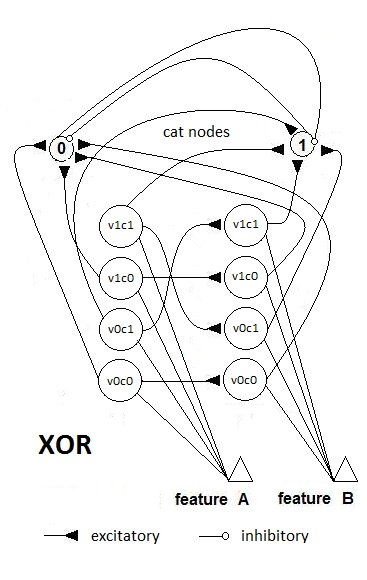 | Figure 27. The SHARP neural network after learning the XOR problem. The category clusters have been removed for simplicity. Feature A is the first input of the “gate,” and Feature B is the second input. The only valid values for this problem are 0 and 1 (in a digital view), so there are 2x2 neurons in any feature cluster. Only the paths of the forward excitatory synapses activated are shown |
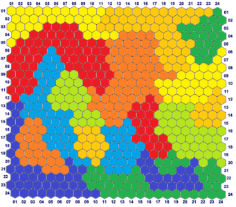
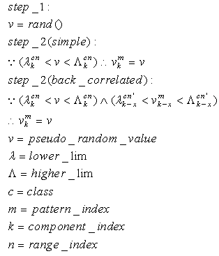
10.2. Random Artificial Database Test
- In the SHARP test framework, we have created a program that can generate example patterns and related validation patterns (with added noise controlled by a NOISE_LIMIT parameter). Any component of any vector is pseudo-randomly generated. For any example vector generated, we have a noisy pattern for the validation purpose.The result is a database of completely random patterns (64 features wide) uniformly distributed to eight classes. Thus, there is no relation between patterns contained in any class, and clusters produced by a Kohonen Map are not distinguishable (Fig. 28).
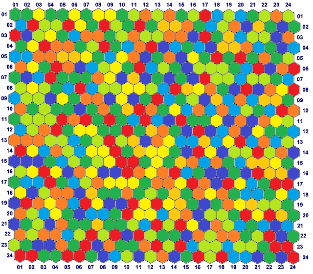 | Figure 28. The output obtained by a SOM trained with a subset of points from the random artificial database. The eight colors refer to the eight different classes associated with the original examples. SOM is unable to create class-related clusters, demonstrating the real random nature of the dataset |
 TEST_2: 5000 training examples + 5000 validation with
  TEST_3: 5000 training examples + 5000 validation with
  Here
Here  is the maximum noise added to any component of the vector
 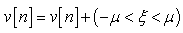 | (73) |
 | (74) |
10.3. Complex Artificial Database Test
- In short, this database differs from the previous one because although patterns are still randomly generated, they are filtered with complex, relational, features-range rules that are associated with specific classes. In other words, these filters accept or reject the randomly generated number depending if it satisfies the rule associated with the current feature and the current class. The rule can be complex, as it can assert multiple ranges whose validity is a function of all or some values assumed by previously generated features.This tool can generate complex databases of patterns associated with multiple classes that can have any arbitrary shape in the space of variables (features). Although the completely random database is the hardest problem for a classifier, a database generated with this system represents a more real classification problem whose complexity can be easily varied (Fig. 29).
 | Figure 29. The SOM representation of the complex database generated with the tool. All patterns have been distributed between eight classes with similarities between couples of classes |
|
 | (75) |
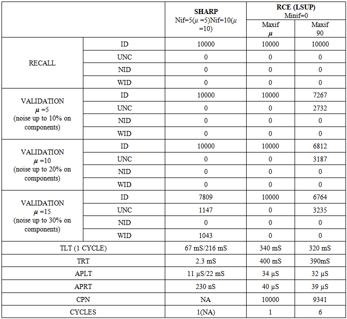
10.4. Circle in the Square Test
- This test, originally proposed by DARPA to check the capability of neural networks, seems to be a “toy problem”; however, it is still a valid method to discover lacks and limits of neural networks in pattern recognition tasks. This problem requires a system to identify which points of a square lie inside and which points lie outside a circle whose area is half that of the square. The intrinsic bi-dimensionality of the problem offers an easily interpretable image of results that would be hidden in a more complex problem.We have compared SHARP with a RCE network. Sometimes, this test can discover conceptual lacks of a pattern recognition algorithm that could not be discovered with more complex tasks. The RCE neural network creates prototypes with large NIF when they are far from edges with a different class (fig. 31). The process subsequent to a “mismatch” condition reduces the NIF of existing prototypes. The NIF of a new prototype is limited by the distance of the nearest prototype owned by a different class. Thus, the number of prototypes grows as a function of the precision requested to recognize the correct class around the points located in the circumference. Few prototypes can roughly recognize points inside and outside the circle. The SHARP neural network, because of its “agnostic resonance”, does not have a mismatch mechanism or a NIF property as intended in RCE. When a pattern is learned, some synapses between any layer and all of the following layers are activated. For any layer representing a feature, a certain number of neurons around the most resonating neuron are involved in the process of synaptic update. The dimension of the region related to synaptic update around the most resonating neuron, is equivalent to NIF in L_SUP mode for an RCE neural network. The SHARP model has prototypes distributed on the entire set of feature layers as a chain of synapses activated by a “systolic Hebb” learning process. These “systolic prototypes” can be overlapped (Fig. 30), so an input pattern can activate more than one category. The synapses that interconnect subsequent feature clusters and synapses that connect the feature layers with the category clusters are analogically activated as a function of the distance from the most resonating neuron. In this way, the contributions to activation of a category neuron is weighted, and conflicting recognitions almost always have different strengths. The WTA mechanism in the category layer substitutes at run-time the “mismatch process” of the RCE, resolving confliction recognitions.
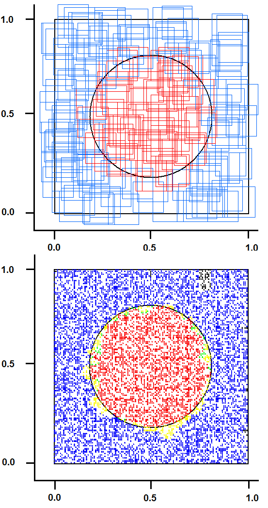 | Figure 30. The result of “Circle in the square test” with SHARP. On the upside: entangled prototypes (200 examples learned). On the downside: 10,000 points recognized (yellow/green = uncertainty/error, black(except contour) = not identified) |
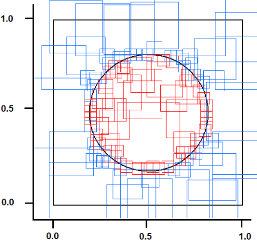 | Figure 31. The prototypes for the “Circle in the square” test of a RCE neural network in L_SUP mode |
11. Technological Considerations
- SHARP can perform one shot learning and recognition by simply addressing synaptic values stored in memory. In this paragraph, we analyze the performance of the network compared with a RCE-like algorithm in a pattern recognition problem.The main problem of RCE and RBF networks is that their algorithms must compare the input pattern with all of the prototypes stored in their database. This operation can be very time consuming when the number of prototypes is huge and the algorithm is executed in a serial computer. In this case, a real-time performance requires the use of SIMD processors. Such processors can compute, in a parallel way, the Euclidean distance or L1 distance between the input pattern and many prototypes. The number of prototypes that can be analyzed at the same time depends on the processor type and its scalability, as most of them can be connected in daisy chain. There are also neural chips implementing neural networks in a RBF-like manner, which can be connected in a daisy chain. Most chips of this type are laboratory units whereas the Cognimem CM1K is a commercial version that embeds 1000 prototypes and allows many chips to be connected in a daisy chain.We have proposed an algorithm that can be executed in real time in a serial computer completing the recognition in a time that is independent of the number of prototypes stored in the network (Fig. 32). Furthermore, the software simulation algorithm requires only sequential readings of synaptic values from memory in lieu of complex computations. The biggest demand of resources is only related to the memory required to store synaptic values. The number of “systolic synapses” between sequential feature clusters grows rapidly (on a factorial basis) with the number of features managed by the network. The synapses between feature clusters and category clusters grow linearly with the number of features and the number of classes.
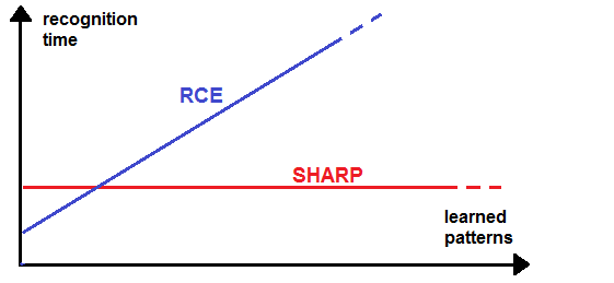 | Figure 32. The recognition time required by SHARP and that required by an RCE in a Von Neumann computer |
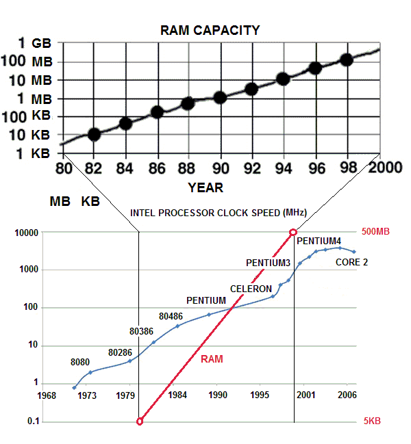 | Figure 33. The growth of clock frequency and the growth of ram capacity in the last twenty years. The growth of memory has been 1000 times the growth of clock frequency |
 | (76) |
 | (77) |
 | (78) |
 | (79) |
 | (80) |
|
11.1. Parallel Hardware Implementation
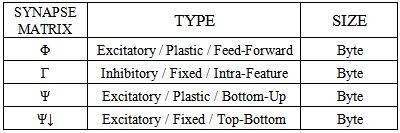
- SHARP can be efficiently implemented on FPGA (Field Programmable Gate Array) or multiple instances of a very simple microcontroller together with distributed fast FRAM (Ferromagnetic Random Access Memory). We have designed, at a higher level, a hardware platform intended to maximize parallelization of the recognition process. We have one FRAM bank, for any couple of features, which stores synaptic connections between couples of layers. Actually, this FRAM stores synaptic connections between the neurons associated to particular features and neurons associated to other features.The project has been optimized to demonstrate that by implementing SHARP in hardware, it is possible to obtain fully parallel huge neural networks with very limited digital electronic resources.The principal constraint in parallelizing the process is the distribution of memories dedicated to a specific feature or group of features. The management of memories could be implemented in a single large FPGA or one small FPGA (or CPLD) / uP for any memory block.The other solution is using a single, very simple uP or CPLD for any FRAM (or FLASH) block managing one feature or a small group of features. The result is a scalable multi-modules system that can be adapted to the pattern dimensionality.The architecture is shown in Fig. 34, where it is possible to distinguish the distribution of operations and synapses management between processing elements. In this system, the features are fed serially in the systolic chain of the modules composed of one CPLD and one FRAM memory. This type of hardware implementation is proposed as a low-cost, scalable solution for a cortical processor.
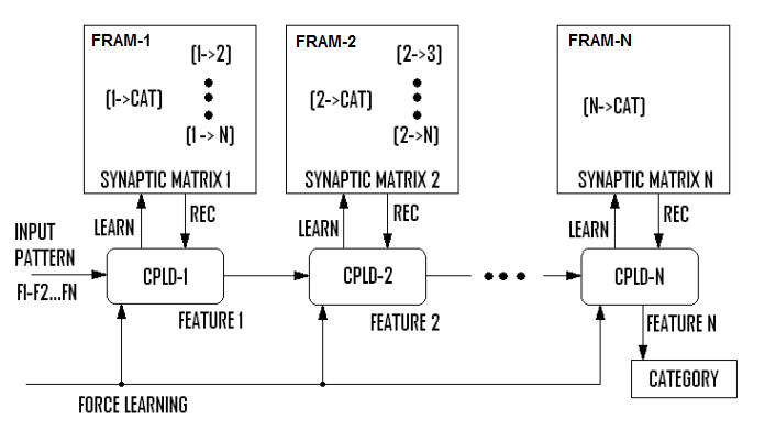 | Figure 34. The hardware implementation with stages composed of a CPLD and a flash memory. In this picture, each stage manages one feature; thus, the parallelism and the speed performance are maximized |
12. Conclusions and Future Work
- We have presented a novel, biology-inspired neural network model that integrates the firing of neurons.We have analyzed the rough biological plausibility of the described paradigm and its spiking neurons models. Then, we have analyzed the issues related to its digital software implementation. Our target has been to find an algorithm respecting the architectural and behavioral characteristics of the proposed paradigm, but that could be very efficiently executed in a typical Von Newman machine. This model is strongly based on the use of memory, but it requires low or almost null computational power. The algorithm is executed in real time on Von Newman processors with performance independent of the number of stored prototypes. In this paper, we have analyzed how the proposed algorithm can be considered a “brick” of a more complex hierarchical structure, considering many other potential analogies with biological systems.We have compared the performance of this algorithm with the classical RCE and RBF. We have also analyzed the project of a possible implementation of such algorithm on commercial hardware to maximize the recognition speed. Currently, we are working on algorithms that could automate the PCS. Furthermore, we plan to work on cognitive systems built on the MOSAIC framework with SHARP modules. The design of a scalable, digital, asynchronous chip working as a “cortical processor” will be the second target of future research.
References
| [1] | Nowotny T, Huerta R, Abarbanel HD, Rabinovich MI. Self-organization in the olfactory system: one shot odor recognition in insects. BiolCybern. 93(6):436-46, 2005. (2003). |
| [2] | Sachse, S. and C. G. Galizia (2002). "Role of Inhibition for Temporal and Spatial Odor Representation in Olfactory Output Neurons: A Calcium Imaging Study." J Neurophysiol 87(2): 1106-1117. |
| [3] | Paolo Arena, Luca Patané, Pietro Savio Termini (2012): Learning expectation in insects: A recurrent spiking neural model for spatio-temporal representation. Neural Networks 32: 35-45 (2012). |
| [4] | Izhikevich E.M. (2003) Simple Model of Spiking Neurons. IEEE Transactions on Neural Networks, 14:1569- 1572. |
| [5] | Izhikevich E.M. (2001) Resonate-and-Fire Neurons. Neural Networks, 14:883-894. |
| [6] | Llinas RR 1988 - The intrinsic electrophysiological properties of mammalian neurons: insights into central nervous system functionDec 23;242(4886):1654-1664, Science— id: 9930, year: 1988, vol: 242, page: 1654, stat: Journal Article. |
| [7] | W. Maass. (1996) On the computational power of noisy spiking neurons. InAdvances in Neural Information Processing Systems, D. Touretzky, M. C. Mozer, and M. E. Hasselmo, editors, volume 8, pages 211-217. MIT Press (Cambridge), 1996. |
| [8] | W. Maass. (1997) Networks of spiking neurons: the third generation of neural network models. Neural Networks, 10:1659-1671, 1997. |
| [9] | Fred Rieke, David Warland, Rob de Ruyter van Steveninck, William Bialek (1999) -Spikes: Exploring the Neural Code - Bradford Book. |
| [10] | J. Gautrais, S. Thorpe (1998) Rate coding versus temporal order coding: a theoretical approachBiosystems 48 (1), 57-65. |
| [11] | Bressler S.L. (1995) Large-scale cortical networks andcognition. Brain Res Rev 20:288-304. |
| [12] | Bressler S.L. (2002) Understanding cognition through large-scale cortical networks. Curr Dir Psychol Sci 11:58-61. |
| [13] | Bressler S.L., Tognoli E. (2006) Operational principles of neurocognitive networks. Int J Psychophysiol 60:139-148. |
| [14] | Cerf et al (2010), On-line, voluntary control of human temporal lobe neurons. Nature, October 28, 2010. doi:10.1038/nature09510. |
| [15] | Gelbard-Sagiv et al. 2008Internally Generated Reactivation of Single Neurons in Human Hippocampus During Free Recall-Published Online September 4 2008Science-3-October-2008: Vol. 322 no. 5898 pp. 96-101 - DOI: 10.1126/science.1164685. |
| [16] | Kreiman, Koch, Fried (2000) - Category-specific visual responses of single neurons in the human medial temporal lobe - Nature Neuroscience3, 946 - 953 (2000) - doi:10.1038/ 78868. |
| [17] | Quian Quiroga, R., Reddy, L., Kreiman, G., Koch, C. & Fried, I. (2005).Invariant visual representation by single neurons in the human brain. Nature, 435:1102–1107. |
| [18] | Quian Quiroga, R., Kreiman, G., Koch, C. & Fried, I. (2008). Sparse but not “Grandmother-cell” coding in the medial temporal lobe. Trends in Cognitive Science, 12, 3, 87–94. |
| [19] | Quian Quiroga, R., Kraskov, A., Koch, C., & Fried, I. (2009). Explicit Encoding of Multimodal Percepts by Single Neurons in the Human Brain.Current Biology, 19, 1308–1313. |
| [20] | Quian Quiroga, R. & Kreiman, G. (2010a). Measuring sparseness in the brain: Comment on Bowers (2009). Psychological Review, 117, 1, 291–297. |
| [21] | Quian Quiroga, R. & Kreiman, G. (2010b). Postscript: About Grandmother Cells and Jennifer Aniston Neurons. Psychological Review, 117, 1, 297–299. |
| [22] | Viskontas, I., Quian Quiroga, R. & Fried, I. (2009). Human medial temporal lobe neurons respond preferentially to personally relevant images. Proceedings of the National Academy Sciences, 106, 50, 21329-21334. |
| [23] | Asim Roy (2012) Discovery of Concept Cells in the Human Brain – CouldIt Change Our Science? –Natural Intelligence Vol.1 Issue.1 INNS magazine. |
| [24] | Barlow, H. (1972). Single units and sensation: A neuron doctrine for perceptual psychology. Perception, 1, 371–394. |
| [25] | Barlow, H. (1995). The neuron doctrine in perception. In The cognitive neurosciences, M. Gazzaniga ed., 415–436. MIT Press, Cambridge, MA. |
| [26] | Gross, C. (2002). Genealogy of the grandmother cell. The Neuroscientist, 8, 512–518. |
| [27] | Baars, Bernard J. (1988), A Cognitive Theory of Consciousness (Cambridge, MA: Cambridge University Press). |
| [28] | Baars, Bernard J.(1997), In the Theater of Consciousness(New York, NY: Oxford University Press). |
| [29] | Baars, Bernard J. (2002) The conscious access hypothesis: Origins and recent evidence. Trends in Cognitive Sciences, 6 (1), 47-52. |
| [30] | J.A. Reggia – Neural Networks, 2013 – Elsevier The rise of machine consciousness: Studying consciousness with computational models. |
| [31] | Baars, B. J., & Franklin, S. An architectural model of conscious and unconscious brain functions: Global Workspace Theory and IDA. Neural Networks (2007), doi:10.1016/j.neunet.2007.09.013. |
| [32] | H.T Kung. Why Systolic Architectures? January 1982 37 c3 1982 IEEE. |