1. Introduction

PLSR is a latent variable based multivariate statistical method that is a combination of PLS and multiple linear regression. It accounts for small sample size, large number of predictor variables, correlated variables and several response variables. The aim of PLS is to constitute latent variables (components) that explain most of the information (variability) in the descriptors that is useful for predicting responses while reducing the dimensionality by using fewer latent variables than the number of descriptors. It can be understood from various perspectives-a way to compute generalized matrix inverses, a method for system analysis and pattern recognition as well as learning algorithm (Martens [11]). For the history of PLS and about PLS regression see Geladi [5] and Höskuldsson [7].

A nonlinear extension of the PLS (partial least squares regression) method is firstly introduced in Frank [4]. A lot of PLS methods were developed in the literature. The activation functions of artificial neural networks are used in PLS method. Because the activation functions provide highly nonlinear transformations, they solve multicollinearity problem. Moreover, PLS method has non-linear modeling ability. Qin and McAvoy [12] propose non-linear PLS method based on feed forward artificial neural networks whereas Yan et al. [18] propose non-linear PLS algorithm based on radial bases activation functions, Zhou et al. [19] propose non-linear PLS method based on logistic activation function and particle swarm optimization methods. Xufeng [13] suggests different non-linear PLS algorithm that differently used feed forward neural networks. Alvarez-Guerra et al. [2] compared Counter propagation neural network and PLS-DA algorithm. Ildiko and Frank [8] proposed a different non-linear PLS algorithm.

In this study, the method of Qin and McAvoy [12] was altering and making a suggestion of a new nonlinear PLS method which is based on Elman feedback artificial neural networks. The paper is organized as follows. In Section 2, frequently used NIPLAS algorithm and the algorithm of Qin ve McAvoy [12] were summarized briefly. Section 3 forms from the brief summary of feedback and feed forward artificial neural networks. In Section 4, the proposed method was introduced. In Section 5, the proposed method was compared with the other methods lie in literature by making an application. In the last section, the results of the analysis were discussed.

2. Linear and Nonlinear Partial Least Squares Regression (PLSR)

PLS method is usually presented as an algorithm to extract latent variables. It creates orthogonal latent variables using different algorithms. The choice of algorithms depends strongly on the shape of the data matrices to be studied (Lindgren, et al. [10]). An often used algorithm is the NIPALS (Non-Linear Iterative Partial Least Squares) algorithm often referred to as the ‘classical’ algorithm. The development of algorithm was initiated by H. Wold [14, 15] and later extended by S. Wold [16, 17] (Lindgren et al., [10]).

The basic algorithm for PLS regression was developed by Wold [14, 15]. The starting point of the algorithm is two data matrices and without any assumptions about their dimensions (N, M or K). is , is where N also represents the number of rows (observations), M also represents the number of columns (predictors), and K is the number of response variables. The standard procedure in PLS method is to centered and scaled matrices by subtracting their averages and dividing their standard deviations. The PLS regression method is an iterative method except on single y variable.

In this study, NIPALS algorithm was performed in analysis. This algorithm can be explained as follows: It starts with the centered and scaled X and Y matrices as and . NIPALS algorithm compose of two loops. The inner loop is used to attain latent variables. The corresponding weight vectors w and c for latent variables are obtained by multiplying the latent variables through the specific matrix as and . u is taken as the first column or column with the biggest variance of Y matrix and w and c are scaled to length 1. t latent variable is obtained as . New u latent variable is defined as . Then a convergence is tested on the change in u. If convergence has been reached the outer loop is used sequentially to extract p loading vectors from X matrices with the new pairs of latent variables. Otherwise, this loop is repeated until a convergence is reached. Loadings are obtained as . In this loop, it is possible to calculate the new t as . In this algorithm a regression model between latent variables is written as and named as inner model. Here b is the regression coefficient of inner relation and computed by . Loadings are calculated to obtain the residual matrices that will be used in the next iteration as and . In these equations the subtracted parts represent decomposition of matrices X and Y into biliner products and named as outer model. These residual matrices are used to obtain new t and u latent variables. The whole set of latent variables has been found when E residual matrix became a null matrix. For more information look (Geladi et al., [6]).

An neural network partial least square (NNPLS) modeling approach which was proposed by Qin et al. [12] was considered in this study. They proposed an NNPLS modeling approach by keeping the outer relation in linear PLS while using neural networks as the inner regressors: . Here, stands for the nonlinear relation represented by a neural network. h and r_h represents iteration number and residual.

3. Neural Networks

Artificial neural network is a data processing mechanism generated by the simulation of human nerve cells and nervous system in a computer environment. The most important feature of artificial neural network is its ability to learn from the examples. Despite having a simpler structure in comparison with the human nervous system, artificial neural networks provide successful results in solving problems such as forecasting, pattern recognition and classification.

Although there are many types of artificial neural networks in literature, feed forward and Elman feedback artificial neural networks are frequently used for many problems. Feed forward artificial neural networks consist of input layer, hidden layer(s) and output layers. An example of feed forward artificial neural network (FFANN) architecture is shown in Figure 1. Each layer consists of units called neuron and there is no connection between neurons which belong to same layer. Neurons from different layers are connected to each other with their weights. Each weight is shown with directional arrows in Figure 1. Bindings shown with directional arrows in feed forward artificial neural networks are forward and unidirectional. In literature, many studies on forecasting use single neuron in output layer. Single activation function is used for each neuron in hidden layer and output layer of feed forward artificial neuron network. Inputs incoming to neurons in hidden and output layers are made up multiplication and addition of neuron outputs in the previous layers with the related weights. Data from these neurons pass through the activation function and neuron output are formed. Activation function enables curvilinear match-up. Therefore, non-linear activation functions are used for hidden layer units. In addition to a non-linear activation function, linear (pure linear) activation function can be used in output layer neuron.

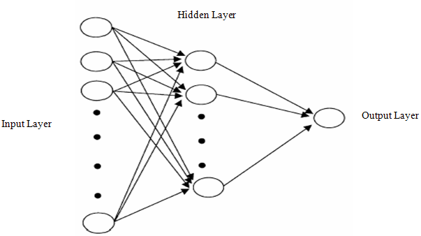Figure 1. Multilayer feed forward artificial neural network with one output neuron

In feed forward artificial neural networks, learning is the determination of weights generating the closest outputs to the target values that correspond with the inputs of artificial neural network. Learning is achieved by optimizing the total errors with respect to weights. There are several types of training algorithms in literature used for learning of feed forward artificial neural networks. One of the widely used training algorithms is Levenberg-Marquardt (LM) (Levenberg, [9]) algorithm which was also used in this study.

Elman artificial neural network is one of the important artificial neural network type used in prediction. Elman neural network, which has the simplest structure among feedback artificial neural networks types, was first proposed by Elman [3]. Elman feedback artificial neural networks consist of input layer, hidden layer, context layer and output layer. Context layer provides a step-delayed feedback mechanism which shows hidden layer output to network as input thus enabling artificial neural network learning with more information. An example of Elman artificial neural network architecture is shown in Figure 2.

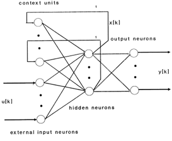Figure 2. Elman recurrent artificial neural network

4. Proposed Method

Most of the real-life data sets rarely have linear structure. For that reason nonlinear methods are essential to use. Therefore multiple nonlinear methods have been proposed along with linear PLS.

In the proposed method in Qin and McAvoy [12] the inner model was formed with feed forward artificial neutral network distinctively from linear PLS method. In this study, Elman feedback artificial neural network was used in generating inner model. It is known in literature that Elman artificial neural network produce better results than feed forward artificial neural network (Aladağ et al. [1]). The algorithm of the proposed method was given as below.

Step 1. Scale X and Y to zero-mean and one variance. Let 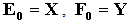and h=1.

Step 2. For each factor h, take .

Step 3. PLS outer transform:

in matrix X: , normalize to norm 1.

• in matrix Y: , normalize to norm 1.

, Iterate this step until it converges.

Step 4. Calculate the X loadings and rescale the variables:

, normalize

, .

Step 5. Find inner network model: train inner network such that the following error function is minimized by Levenberg-Marquardt method.

Here, is the output of the Elman artificial neural network. For example, if the number of hidden layer was 1, Elman Neural Network that was used in obtaining was given in Figure 3. The architecture of Elman type artificial neutral network was given in Figure 3 and logistic activation function was used in all neurons of Elman type artificial neutral network. Also, the number of hidden layer unit has been determined obtained by trial-error method.

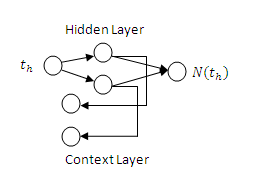Figure 3. Inner Model

Step 6. Calculate the residuals for factor h:

for matrix X,

for matrix Y,

where .

Step 7. Let h=h+1, return to Step 2 until all principal factors are calculated.

In the proposed method, FFANNs are used in every iteration of algorithm. Because of this, a lot of FFANN were employed in the proposed method. Convergence of FFANN is provided by using 100 iteration at least for each neural network.

5. Application

The data used in this study was about a total of 30 young football players enrolled in the league of “Football Players who are Candidates of Professional Leagues”. In this data set, the number of observation units (young football players) is 30. Explanatory variables are taken from the right side and left side of the body such as width of the circumference for right and left arm, width of circumference for right and left forearm, width of circumference for right and left hand. These calculations were done also for thigh, knee, hip and foot. At the same time the length of the arm, forearm, hand, thigh, foot and leg for the right and left side of the body was calculated. The thickness of skinfold of abdomen, the skinfold of triceps, subscapular, biceps, patella and extremities values were taken, too. So the number of explanatory variables is about 73.

The number of dependent variables is 2. They are vertical and broad jumping with two legs refer to y1 and y2, respectively. So, X: , Y: . Vertical jumping was measured in centimeter, broad jumping was measured in meter. Length and circumference measurements were measured in centimeters and skinfold was measured in millimeter.

Randomly selected 27 observations were used to obtain the models. 3 observations were used as test set (n_test=3). That is, 27 observations were used in modeling, 3 were used in prediction. As a comparison criterion RMSE (root mean square error) was used. RMSE values for test set by predicting with PLSR method appear in Table 4.

Firstly, prediction was made with FFANN method in MATLAB R2011b. Input number of FFANN is the number of explanatory variables. On the other hand, the numbers of hidden layer neurons vary between 1 and 73, the 73 different FFANN architectures are used for obtaining predictions. The FFANN was trained by using Levenberg-Marquardt algorithm with 500 maximum number of iterations. The best result of FFANN is the architecture (73-8-2) which has 73 inputs, 8 hidden layer neurons and two outputs.

Table 1. Obtained RMSE Results

6. Conclusions

Nonlinear partial least square methods have been very popular in recent years. In this study, we proposed new nonlinear PLS method based on Elman neural network. In the proposed method, the inner model is Elman recurrent neural network. The proposed method improves Qin and McAvoy [12] method. The proposed method was applied to data set of “30 young football players enrolled in the league of Football Players who are Candidates of Professional Leagues” and compared with some PLS methods. As a result of application, we show that the proposed method outperforms linear PLS (Nipals), feed forward artificial neural netwroks and Qin and McAvoy [12] method according to RMSE criterion.

ACKNOWLEDGEMENTS

This study was financially supported by Ondokuz Mayıs University as a BAP Project.