1. Introduction

Linear regression method is a classic statistical method. Linear regression method has a lot of assumptions like other statistical techniques. These assumptions are not realistic in the real world application. These assumptions are checked by statisticians. If they are not suitable for data, advanced statistical techniques are applied to the data. Ridge regression is a kind of advanced statistical technique. When data has multicollinearity problem, ridge regression technique can give a solution for data. In this study, a new ridge regression method is introduced.

Consider a linear multiple

(1)

where Y is the vector of observations of the dependent variable, X is the matrix of observations of explanatory variables with full rank p, is the vector of unknown parameters and is the vector of random error, where and p shows the number of explanatory variables in the model. It is assumed that each random error has zero mean and a constant variance and that they are uncorrelated.

Moreover it is assumed that the columns of X should not be in a linear dependency of each other.

Let us denote the columns of X as . If there is a relationship

(2)

for a set of numbers such as , not all zero, the relation is called the multicollinearity problem in multiple regression analysis.

Multicollinearity can also cause to produce least squares estimates of ’s which are too large in absolute value.

When the columns of X matrix are centered and scaled the matrix becomes the correlation matrix of the explanatory variables and is the vector of the correlation coefficients of the dependent variable with each explanatory variable. If the columns X are orthogonal, matrix is a unit matrix. In the presence of multicollinearity becomes ill-conditioned which means that it is nearly singular and the determinant of it is nearly zero. Some of the eigenvalues of can also be very near to zero. Some prefer to examine

(3)

which is called as condition number. In this equation λ is the eigenvalues of . Generally if the condition number is less than 100, there is no serious multicollinearity problem. Condition numbers between 100 and 1000 imply moderate to strong multicollinearity and if it exceeds 1000 it indicates that severe multicollinearity exists in the data. The variance-covariance matrix of is determined by

(4)

The diagonal elements of this matrix are called the variance inflation factors (VIF) and are given by

(5)

where is the determination coefficient obtained from the multiple regression of on the remaining regressor variables in the model. If there is a strong collinearity between and any subset of the remaining regressor variable the value of will be close to 1. Therefore is going to be very large and it implies that the variance of is to be large. Briefly speaking the following items can be considered as the multicollinearity diagnostics.

1. The correlation matrix constructed by X

2. The determinant of the matrix of

3. The eigenvalues of

4. VIF values

(Montgomery and Peck [1])

To overcome multicollinearity problem, the ridge regression has been suggested in the literature (Hoerl and Kennard [2], Hoerl et al. [3]). But there is another problem for applying ridge regression such as finding the optimal biasing parameter (k) value. Several methods have been proposed for finding it. These are; Hoerl and Kennard [2], Hoerl et al. [3], Mc Donald and Galarneau [4], Lawless and Wang [5], Hocking [6], Wichern and Curchill [7], Nordberg [8], Praga-Alejo et al. [9], Al Hassan [10], Ahn et al. [11]. And also, Siray et al. [12] proposed an approach to examine multicollinearity and autocorrelation problems.

In this study, a new algorithm of estimating k value by using particle swarm optimization was introduced.

In addition to these studies, there are some studies in the literature about ridge estimation and its estimators. For example, Sakallıoglu and Kacıranlar [14] proposed a new biased estimator for the vector of parameters in a linear regression model based on ridge estimation. Firinguetti and Bobadilla [14] proposed an approach to develop asymptotic confidence intervals for the model parameters based on ridge regression estimates. Tabakan and Akdeniz [15] proposed a new difference – based ridge estimator of parameters in partial linear model. Duran and Akdeniz [16] proposed an estimator named modified jackknifed Liu-type estimator to show its efficiency in ridge regression. Uemukai [17] showed the small sample properties of a ridge regression estimator when there exists omitted variables by inspiring the study of Huang [18]. Akdeniz [19] proposed new biased estimators under the LINEX loss function. And also, there are some combining methods about new estimators such as Alkhamisi [20].

The rest part of the paper can be outlined as below: The second section of the article is about Ridge regression. The methodology of the paper was given in Section 3. The implementation of our proposed method was given in Section 4 and finally, discussions were presented in Section 5.

2. Ridge Regression

(6)

the ridge estimates are introduced as

(7)

where k is a very small constant determined by the researcher Hoerl and Kennard [2]. Gauss Markov theorem states that under the standard assumptions about errors the ordinary least squares estimators (OLS) of the parameters of the model in (1) are unbiased and have the minimum variances. But there is no guarantee that the variance of will be small. For this purpose the ridge estimator estimates with a bias but has a smaller variance than the ordinary least squares estimators’ one. When we look at the mean squared error of we can easily see that

(8)

can be made small than the mean squared error of which is equal to variance of since there is no bias in it.

The ridge estimator can be expressed as a linear transformation of the ordinary least squares estimator as below.

(9)

When we look at the expected value of ridge estimator, we can easily see that it is a biased estimator of .

(10)

The variance-covariance matrix of is

(11)

Let us look at the mean squared error of two estimators to compare them. Since the ordinary least squares estimator is unbiased, the mean squared error will be the variance of the estimator.

(12)

where is the eigenvalues of . Contrarily the mean squared error of ridge estimator is

(13)

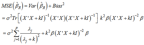Notice from (13) can be made by choosing an optimal k value. Hoerl and Kennard [2] proved that there is nonzero k value for which is less than provided that is bounded. On the other hand the mean squared error based on the ridge estimator is also compound of two parts; one part which is the first term of the right-hand side of (13) decreases and the other increases when k increases. The residual sum of squares based on the ridge estimator can be expressed as below.

(14)

This expression implies that as k increases the sum of squares of residual increases and consequently decreases. Therefore the ridge estimate will not give the best fit to the data necessarily when we are more interested in obtaining a stable set of parameter estimates.

From this point, we face the question how we can find an appropriate value for biasing parameter k. Ridge trace is one of the methods which are used for it. It is a plot of the elements of the ridge estimator versus k usually in the interval (0, 1) (Hoerl and Kennard [21]). Marquardt and Snee [22] suggested using only 25 values of k, spaced approximately logarithmically over that interval. From the ridge trace, the researchers can see that at a reasonable k value the estimates become stable. In this paper for the purpose of comparing the results we just consider the methods of which a brief introduction is given as below.

Hoerl et al. [3] suggested another method for finding k value which is given as

(15)

where and are the ordinary least squares estimates. This method is referred as fixed point ridge regression method. For ease of use we will symbolize this method as FPRRM.

Hoerl and Kennard [23] introduced an iterative method for finding the optimal k value. In this method k is calculated as in below;

(16)

where and are the corresponding residual mean square and the estimate vector of regression coefficients at (t-1)th iteration, respectively. Generally, the initials are chosen the results from the least squares method. The method will be presented here as iterative ridge regression method (IRRM) for abbreviation.

3. Methodology

Finding optimal k value has always been problematic. In recently, genetic algorithm has been used for this purpose such as Praga-Alejo et al. [9] and Ahn et al. [11] did. Praga-Alejo et al. [9] found the optimal k value by minimizing a distance based on VIFs. Ahn et al. [11], differently from Praga-Alejo et al. [9], used SSE as fitness function. Praga-Alejo et al. [9] found the optimal k value as nearly 1 because of regarding the minimizing of only VIF values. On the other hand Ahn et al. [11] found k as nearly zero because they minimize SSE. Consequently when k value is near to 1 the magnitude of the bias of the estimator, therefore SSE is becoming very large as VIF values are less than 10, which means that there is no multicollinearity problem. If k value is very near to zero then SSE is almost near to the result from the least squares but we cannot get any improvement for VIF values. In order to overcome these deficiencies a method which takes into consideration simultaneously both criteria, for finding the optimal kwas proposed. In this study the proposed method firstly finds the k value which make the VIF's smaller, that is, less than 10 and SSE minimum, at the same time. The optimization problem in the proposed method can be constructed as below.

(17)

with subject to:

where MAPE(k) and can be defined as below:

(18)

(19)

Algorithm.

Step 1 The parameters such as pn, etc., are determined. These parameters are as follows:

pn: particle number of swarm

: Cognitive coefficient

: Social coefficient interval

maxt: Maximum iteration number

w: Inertia weight

Step 2 Generate a random initial positions and velocities.

The initial positions and velocities are generated by uniform distribution with (0,1) parameters. Each particle has one velocity and one position which represent k value. represents the position of particle m at iteration t and represents the velocity of the particle m at iteration t.

Step 3 The Fitness function is defined as in (17). Fitness values of the particles are calculated.

Step 4 According to fitness values, Pbest and Gbest particles given in (20) and (21), respectively, are determined.

(20)

(21)

Pbest is constructed by the best results obtained in the related positions at iteration t. Gbest is the best result in the swarm at iteration t.

Step 5 New velocities and positions of the particles are calculated by using the formulas given in (22) and (23).

(22)

(23)

where rand₁ and rand₂ are random numbers which are generated from U(0,1).

Step 6 Repeat from Step 3 to Step 6 until t<maxt.

Step 7. The optimal k value is obtained as Gbest.

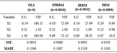
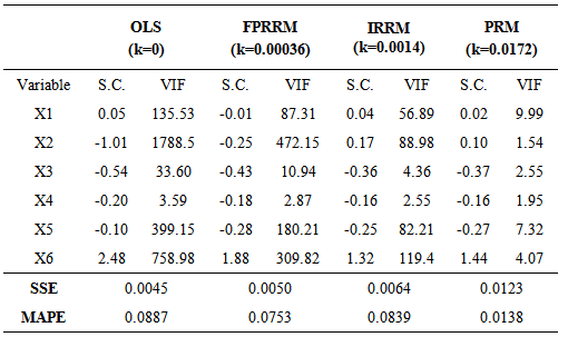
4. Implementation

The proposed algorithm has been experienced on two different and well known real data sets in order to investigate the progress provided by the algorithm. These two data sets are known as “Import Data” and “Longley Data”. Import data has been analyzed by Samprit and Hadi [25]. The variables are imports (IMPORT-Y), domestic production (DOPROD-X1), stock formation (STOCK-X2) and domestic consumption (CONSUM-X3), all measured in billions of French francs for the years 1949 through 1959. Longley’s data set is a classic example of multicollinear data (Samprit and Hadi [25]).

Import data and Longley data have been solved by using fixed point method (FPMRRM) (Hoerl et al. [3]), iterative method (IPRRM) (Hoerl and Kennard [23]) and the algorithm proposed in this paper. In the algorithm PSO parameters were chosen as pn=30, w=0.9, and max t =100. In the iterative ridge method the stopping criteria has been chosen as . The results were presented in the Table 1 and Table 2, respectively.

Table 1. The Coefficient Estimates, VIF Values and SSE and MAPE Obtained From OLS, FPRRM, IRRM and PRM for Import Data

Table 2. The Coefficient Estimates, VIF Values and SSE and MAPE Obtained from OLS, FPRRM, IRRM and PRM for Longley Data

In the tables given below; PRM represents the proposed ridge method and SC represents the Standardized Coefficients.

As it can be seen from these tables, the k value obtained from our algorithm has provided most optimal VIF values which are smaller than 10. It implies there is no more multicollinearity problem in the data. k values from the other techniques have made VIF values smaller than those from ordinary least squares method, but they are not sufficiently small, still. Moreover the value of MAPE has been reduced by the proposed algorithm, comparing with MAPE from OLS.

5. Discussion

In the regression analyze, the variances of the estimated parameters and the residual sum of squares as a goodness of fit measure are desired to be very small. When there exists multicollinearity problem unfortunately the property of being minimum variances of the ordinary least squares estimates does not satisfy anymore. The ridge regression is one of the remedy of multicolinearty problem and it can be employed very often in the literature.

However finding k is another problem while implying ridge regression. The existing methods for finding k value in the literature are based on either reducing VIF values or minimizing the residual sum of squares. In this study the proposed algorithm for finding k value is based on both reducing VIF values and minimizing the residual sum of squares at a time. Since the objective function introduced in the paper is a piecewise function, classical optimization techniques are not suitable.

Therefore the particle swarm optimization has been used for solving optimization problem in this study. It can be actually possible to use other artificial intelligence optimization techniques. Furthermore, we might think about finding different k values for each explanatory variable in future works.