Vincent A. Akpan1, Reginald A. O. Osakwe2
1Department of Physics Electronics, The Federal University of Technology, P.M.B. 704, Akure, Ondo State, Nigeria
2Department of Physics, The Federal University of Petroleum Resources, P.M.B. 1221 Effurun, Delta State, Nigeria
Correspondence to: Vincent A. Akpan, Department of Physics Electronics, The Federal University of Technology, P.M.B. 704, Akure, Ondo State, Nigeria.
| Email: |  |
Copyright © 2014 Scientific & Academic Publishing. All Rights Reserved.
Abstract
A novel technique for the nonlinear modeling and online prediction of incoming influent characteristics of an activated sludge wastewater treatment (AS-WWTP) is presented in this paper. The nonlinear modelling and online prediction in the presence of disturbances is achieved using an online adaptive recursive least squares (ARLS) algorithm to the nonlinear model identification formulated in this paper. The performance of the proposed ARLS algorithm is compared with the so-called incremental backpropagation (INCBP) which is also an online identification. These two algorithms are validated by one-step, five-step ahead prediction methods as well as the Akaike’s method to estimate the final prediction error (AFPE) of the regularized criterion. Furthermore, the validation results show the superior performance of the proposed ARLS algorithm in terms of much smaller prediction errors when compared to the INCBP algorithm. The results from the incoming influent characteristics predictions show three scenarios, namely: high toxic, low toxic and acceptable toxic levels of the incoming influent. The proposed techniques and algorithms can be adapted and deployed for the modeling and prediction of an incoming influent (sewage) for industrial WWTP management systems.
Keywords:
ARLS, Artificial neural network (ANN), AS-WWTP, Benchmark simulation model No. 1 (BSM #1), INCBP, Influent (sewage) characteristics
Cite this paper: Vincent A. Akpan, Reginald A. O. Osakwe, Online Prediction of Influent Characteristics for Wastewater Treatment Plants Management Using Adaptive Recursive NNARMAX Model, American Journal of Intelligent Systems, Vol. 4 No. 3, 2014, pp. 107-130. doi: 10.5923/j.ajis.20140403.03.
1. Introduction
The wastewater treatment is extremely important for humans as well as animals and plants. Generally, the wastewater is exposed to different processes which can remove most of the pollutants such as organic substances, ammonium, phosphorus, nitrogen and other residuals from industrial environment and urban or rural communities. Excess nitrogen and phosphorus in surface waters and nitrogen in groundwater causes eutrophication (i.e. excess algae growth) in surface waters and causes health related problems in humans and livestock as a result of high intake of nitrogen in its nitrate form. Also the effluent quality from industrial wastewater treatment plants are now subjected to tighter regulation as a result of these nutrients as well as nitrogen and phosphorus in both public and receiving waters.Wastewater treatment processes are very complex, strongly nonlinear and characterized by uncertainties regarding its parameters [1]. In previous studies, the complete modelling of the WWTP process has been a challenging problem and thus researchers decomposes the WWTP process into two parts namely; the biological reactors and the settler. Also, attempts have been made to use the well-celebrated neural network due to its approximating capability for the complete modeling of the WWTP process as a single multivariable system i.e. combining the biological reactors and the settler as one entity. In this study, attempt is made to obtain a neural network model of an incoming influent (sewage) that will be used to predict the influent characteristics in order to take decisions on the channelling of the incoming influent to the appropriate channel for the proper management of an AS-WWTP process.The activated sludge process was developed in England in 1914 by Arden and Lockett [2] and was so named because it involved the production of an activated mass of microorganisms capable of aerobically stabilizing a waste. The activated sludge process has been utilized for treatment of both domestic and industrial wastewaters for over half a century. This process originated from the observation made a long time ago that whenever wastewater, either domestic or industrial, is aerated for a period of time, the content of organic matter is reduced, and at the same time a flocculent sludge is formed. Microscopic examination of this sludge reveals that it is formed by a heterogeneous population of microorganisms, which changes continually in nature in response to variation in the composition of the wastewater and environmental conditions. Microorganisms present are unicellular bacteria, fungi, algae, protozoa, and rotifers.Wastewater normally contains thousands of different organics and a measurement of each individual organic matter would be impossible rather a different collective analyses are used which comprise a greater or minor part of the organics. Activated sludge wastewater treatment processes are difficult to control because of their complexity; nonlinear behaviour; large uncertainty in uncontrolled inputs and in the model parameters and structures, and multiple time scales of the dynamics and multivariable input-output structure. The activated sludge process aims to achieve, at minimum costs, a sufficiently low concentration of biodegradable in the effluent together with minimal sludge production; and this is achieved through efficient control of the process. The first control opportunity in ASWWTP is in regulating the influent flow-rate which implies that control issues in wastewater treatment facilities pertain primarily to aeration control for energy usage and satisfying process demands [3].While the dissolve oxygen concentration is considered as the most important control parameter in activated sludge process (ASP), the control of dissolved oxygen level in the ASWWTP reactors plays an important role in the operation of the plant. DO concentration control of the ASP has been recognized as a rewarding and meaningful control, both from economical and biological point of view [1]. Several research papers have been published on how to model and control WWTPs [4]–[8]. The review of most research papers in this area considers modeling and control issues in wastewater treatment facilities in terms of aeration control for energy usage and satisfying process demands. Unlike [3], the view of this paper, however, is that the first control opportunity in ASWWTP should be on the prediction of the characteristics of the incoming influent before the modeling and control of the complete WWTP to determine the toxic content level of the incoming influent.The sensors and actuators employed for parameter measurements and control of WWTP processes are very expensive; and many researchers have been searching for alternative ways to carry out these measurements [9]. The life span the sensors are usually shortened due to the characteristics and quality of the incoming influent (sewage). Thus, it becomes imperative to know in advance the characteristic of the incoming influent to determine the degree of pretreatment or disposal of the incoming influent while bearing in mind the international regulations on the disposal of waste in receiving waters.The objective of this paper is directed towards the online prediction of influent characteristics of the incoming sewage for the proper management of WWTPs. The paper is organized as follows. Section 2 presents the WWTP process description. The neural network-based adaptive recursive least squares (ARLS) algorithm is summarized in Section 3. The online prediction problem of the influent characteristics is formulated and integrated with the proposed neural network identification scheme is given in Section 4. The implementation of the online prediction of the influent characteristics and the simulation results are presented in Section 5. Section 6 concludes the paper with some discussions and future directions.
2. The AS-WWTP Process Description
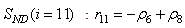
With the tight effluent requirements defined by the European Union and to increase the acceptability of the results from wastewater treatment analysis, the generally accepted COST Actions 624 and 682 benchmark simulation model no. 1 (BSM1) model is considered [1], [4]–[8]. The BSM1 model uses eight basic different processes to describe the biological behaviour of the AS-WWTP processes. The combinations of the eight basic processes results in thirteen different observed conversion rates as described in Appendix A. These components are classified into soluble components  and particulate components
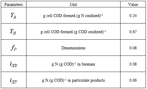
  . The nomenclatures and parameter definitions used for describing the AS-WWTP in this work are given in Table 1. Moreover, four fundamental processes are considered: the growth and decay of biomass (heterotrophic and autotrophic), ammonification of organic nitrogen and the hydrolysis of particulate organics.
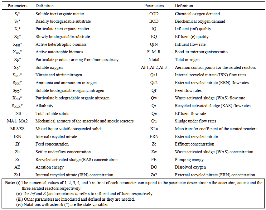 | Table 1. The AS-WWTP Nomenclatures and Parameter Definitions |
The reference model of biochemical reactions in the bioreactors is the activated sludge model no.1 (ASM1) [1], [4]–[8]. The success of this model has prompted widespread interest in biochemical modeling of wastewater in both academia and industry. The overall WWTP model consists of two main parts: the hydraulic model, which represents reactor behaviour, flow rates and recirculation; and the second primary component of WWTP model, is the activated sludge model, which portrays microbial growth, death and nutrient consumption. These models are necessarily approximations to the vast number of biological processes occurring in each bioreactor. Selection of the proper model allows adequate description of those processes most relevant to a particular WWTP. The development of accurate models is a prerequisite for applying model predictive control techniques for the whole process control and dynamic optimization.The schematic of a BNR-ASWWTP design with basic control strategies is shown in Fig.1 using the Johannesburg configuration [7], [8] which consists of anaerobic, anoxic and aerobic zones and a secondary settler in a back-to-back scheme with multiple recycle streams [8]. To ensure that plug flow conditions prevail in the bioreactors, the basins are usually partitioned such that back-mixing is minimized. The constructional features and nomenclature of the process is detailed in Appendix C of [8].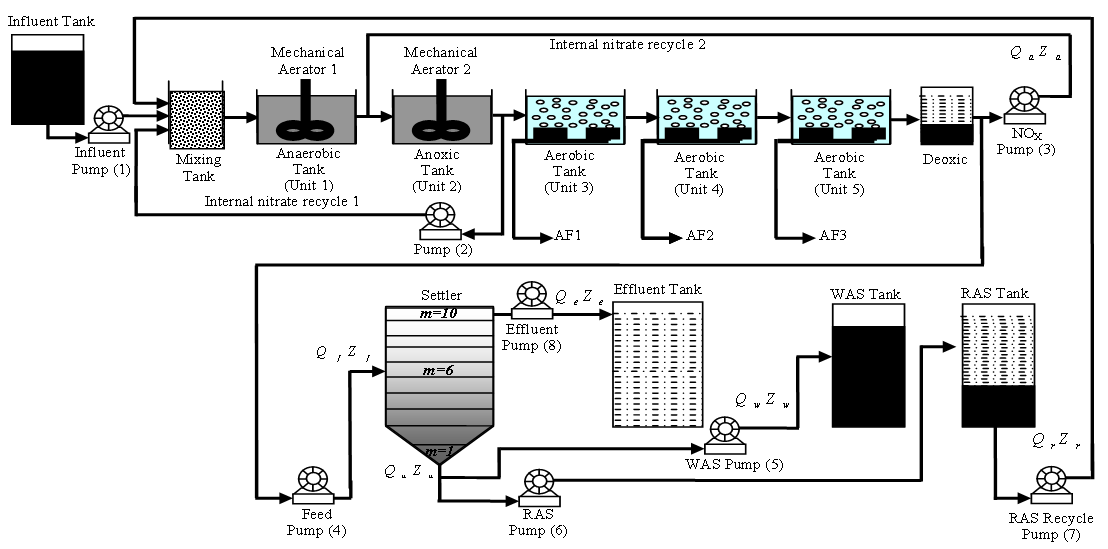 | Figure 1. The schematic of the AS-WWTP process |
The basic mode of operation of the AS-WWTP process is as follows. Organic wastewater is introduced into a reactor where an aerobic bacterial culture is maintained in suspension. The reactor contents are referred to as the mixed liquor. In the reactor, the bacterial culture converts the organic content of the wastewater into cell tissue. The aerobic environment in the reactor is achieved by the use of diffused or mechanical aeration, which also serve to maintain the liquor in a completely mixed regime. After a specified period of time, the mixture of new cells and old cells is passed into a settling tank where the cells are separated from the treated wastewater. A portion of the settled cells is recycled to maintain the desired concentration of organisms in the reactor, and a portion is wasted.
3. The Neural Network Identification Scheme and Validation Algorithms
3.1. Formulation of the Neural Network Model Identification Problem
The method of representing dynamical systems by vector difference or differential equations is well established in systems and control theories [7], [8], [10], [11]. Assuming that a p-input q-output discrete-time nonlinear multivariable system at time  with disturbance
  can be represented by the following Nonlinear AutoRegressive Moving Average with eXogenous inputs (NARMAX) model:
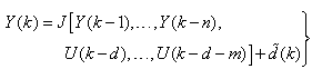 | (1) |
where  is a nonlinear function of its arguments, and
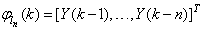
 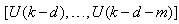 are the past input vector,
  are the past output vector,
  is the current output,
  and
and  are the number of past inputs and outputs respectively that define the order of the system, and
  is time delay. The predictor form of (1) based on the information up to time
  can be expressed in the following compact form as:
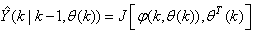 | (2) |
where 
 is the regression (state) vector,
  is an unknown parameter vector which must be selected such that
  is the error between (1) and (2) defined as
 | (3) |
where  in
in  of (2) is henceforth omitted for notational convenience. Not that
  is the same order and dimension as
 .Now, let
  be a set of parameter vectors which contain a set of vectors such that:
 | (4) |
where  is some subset of
  where the search for
  is carried out;
  is the dimension of
  is the desired vector which minimizes the error in (3) and is contained in the set of vectors
 are distinct values of
  ; and
; and  is the number of iterations required to determine the
  from the vectors in
  .Let a set of
  input-output data pair obtained from prior system operation over NT period of time be defined:
 | (5) |
where  is the sampling time of the system outputs. Then, the minimization of (3) can be stated as follows:
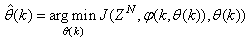 | (6) |
where  is formulated as a total square error (TSE) type cost function which can be stated as:
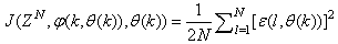 | (7) |
The inclusion of  as an argument in
  is to account for the desired model
  dependency on
 . Thus, given as initial random value of
 and (5), the system identification problem reduces to the minimization of (6) to obtain
 . For notational convenience,
  shall henceforth be used instead of
 .
.
3.2. Neural Network Identification Scheme
The minimization of (6) is approached here by considering  as the desired model of network and having the DFNN architecture shown in Fig. 2. The proposed NN model identification scheme based on the teacher-forcing method is illustrated in Fig. 3. Note that the “Neural Network Model” shown in Fig. 3 is the DFNN shown in Fig. 2. The inputs to NN of Fig. 3 are
 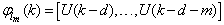 ,
,  and
and 
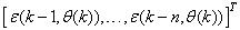 which are concatenated into
  as shown in Fig. 2. The output of the NN model of Fig. 3 in terms of the network parameters of Fig. 2 is given as:
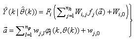 | (8) |
where  and
and  are the number of hidden neurons and number of regressors respectively;
  is the number of outputs,
  and
and  are the hidden and output weights respectively;
  and
and  are the hidden and output biases;
  is a linear activation function for the output layer and
  is an hyperbolic tangent activation function for the hidden layer defined here as:
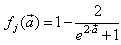 | (9) |
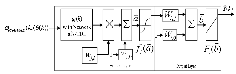 | Figure 2. Architecture of the dynamic feedforward NN (DFNN) model |
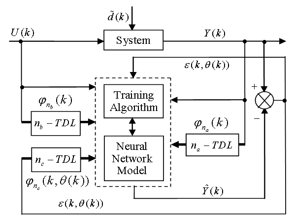 | Figure 3. NN model identification based on the teacher-forcing method |
Bias is a weight acting on the input and clamped to 1. Here,  is a collection of all network weights and biases in (8) in term of the matrices
 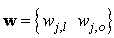 and
and  . Equation (8) is here referred to as NN NARMAX (NNARMAX) model predictor for simplicity.Note that
  in (1) is unknown but is estimated here as a covariance noise matrix,
 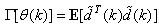 Using
Using , Equation (7) can be rewritten as [5], [6]:
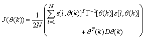 | (10) |
where the second term in (10) is the regularization (weight decay) term [31] which has been introduced to reduce modeling errors, improve the robustness and performance of the two proposed training algorithms.  is a penalty norm and also removes ill-conditioning, where
  is an identity matrix,
  and
and  are the weight decay values for the input-to-hidden and hidden-to-output layers respectively. Note that both
  and
and  are adjusted simultaneously during network training with
  and are used to update
  iteratively. The algorithm for estimating the covariance noise matrix and updating
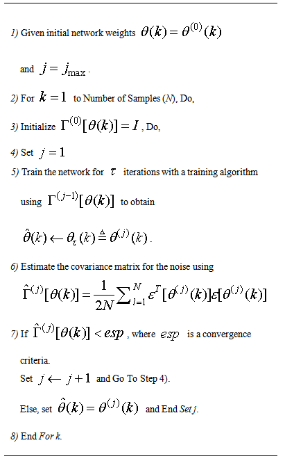
  is summarized in Table 2. Note that this algorithm is implemented at each sampling instant until
  has reduced significantly as in step 7).
Table 2. Iterative algorithm for estimating the covariance noise matrix
 |
| |
|
3.3. Formulation of the Neural Network-Based ARLS Algorithm
Unlike the BP which is a steepest descent algorithm, the ARLS and MLMA algorithms proposed here are based on the Gauss-Newton method with the typical updating rule [7], [8], [10], [11]: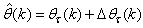 | (11) |
where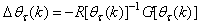 | (12) |
 denotes the value of
  at the current iterate
 is the search direction,
  and
and  are the Jacobian (or gradient matrix) and the Gauss-Newton Hessian matrices evaluated at
  .As mentioned earlier, due to the model
  dependency on the regression vector
 , the NNARMAX model predictor depends on a posteriori error estimate using the feedback as shown in Fig. 2. Suppose that the derivative of the network outputs with respect to
  evaluated at
  is given as [8]:
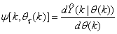 | (13) |
The derivative of (13) is carried out in a BP fashion for the input-to-hidden layer and for the hidden-to-output layer respectively for the two-layer DFNN of Fig. 2. Thus, the derivative of the NNARMAX model predictor can be expressed as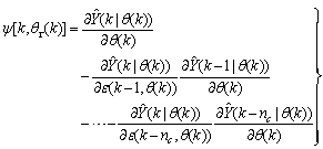 | (14) |
Thus, Equation (14) can be expressed equivalently as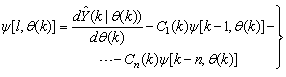 | (15) |
By letting 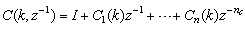 , then (15) can be reduced to the following form
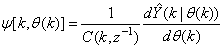 | (16) |
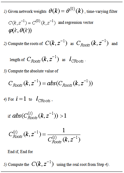
As it can be seen from (16), the gradient is calculated by filtering the partial derivatives with the time-varying filter  which depends on the prediction error based on the predicted output. Equation (16) is the only component that actually impedes the implementation of the NN training algorithms depending on its computation.Due to the feedback signals, the NNARMAX model predictor may be unstable if the system to be identified is not stable since the roots of (16) may, in general, not lie within the unit circle. The approach proposed here to iteratively ensure that the predictor becomes stable is summarized in the algorithm of Table 3. Thus, this algorithm ensures that roots of
  lies within the unit circle before the weights are updated by the training algorithm proposed in the next sub-section.
Table 3. An algorithm for placing the roots of the time-varying filter of the NNARMAX model predictor within the unit circle for stability
 |
| |
|
3.3.1. The Adaptive Recursive Least Squares (ARLS) Algorithm
The proposed ARLS algorithm is derived from (11) with the assumptions that: 1) new input-output data pair is added to  progressively in a first-in first-out fashion into a sliding window, 2)
  is updated after a complete sweep through
  , and 3) all
  is repeated
  times. Thus, Equation (10) can be expressed as [8]:
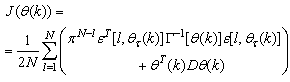 | (17) |
 is the exponential forgetting and resetting parameter for discarding old information as new data is acquired online and progressively added to the set
  .Assuming that
  minimized (17) at time
 then using (17), the updating rule for the proposed ARLS algorithm can be expressed from (11) as:
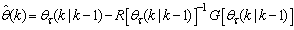 | (18) |
where  and
and  given respectively as:
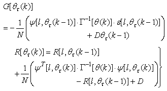 | (19) |
where  is computed according to (16).In order to avoid the inversion of
 , Equation (19) is first computed as a covariance matrix estimate,
  , as
, as 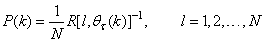 | (20) |
Then, by using the following matrix inversion lemma: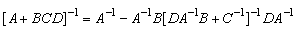 By setting
 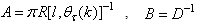 and
and  , Equation (20) can also be expressed equivalently as
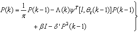 | (21) |
where  is the adaptation factor given by
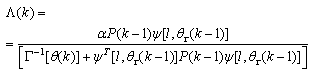 and
and  is an identity matrix of appropriate dimension,
 and
and  are four design parameters are selected such that the following conditions are satisfied [7], [8]:
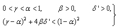 | (22) |
where  in
in  adjusts the gain of the (21),
  is a small constant that is inversely related to the maximum eigenvalue of P(k),
  is the exponential forgetting factor which is selected such that
  and
and  is a small constant which is related to the minimum
  and maximum
  eigenvalues of (21) given respectively as [7], [8]:
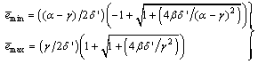 | (23) |
The values of  and
and  in (22) is selected such that
 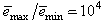 while the initial value of
 , that is
 , is selected such that
 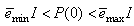 [8].Thus, the ARLS algorithm updates based on the exponential forgetting and resetting method is given from (18) as
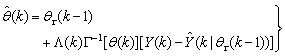 | (24) |
where the second term in (20) is  . Note that after
  has been obtained, the algorithm of Table 2 is implemented the conditions in Step 7) of the Table 2 algorithm is satisfied.
3.4. Proposed Validation Methods for the Trained NNARMAX Model
Network validations are performed to assess to what extend the trained network has approximated and capture the operation of the underlying dynamics of a system and as measure of how well the model being investigated will perform when deployed for the actual process [10]–[12].The first test involves the comparison of the predicted outputs with the true training data and the evaluation of their corresponding errors using (3).The second validation test is the Akaike’s final prediction error (AFPE) estimate [9]–[12] based on the weight decay parameter D in (10). A smaller value of the AFPE estimate indicates that the identified model approximately captures all the dynamics of the underlying system and can be presented with new data from the real process. Evaluating the  portion of (3) using the trained network with
  and taking the expectation
  with respect to
  and
and  leads to the following AFPE estimate [9]–[12]:
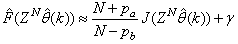 | (25) |
where 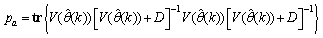 and
and  is the trace of its arguments and it is computed as the sum of the diagonal elements of its arguments,
 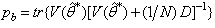 and
and  is a positive quantity that improves the accuracy of the estimate and can be computed according to the following expression:
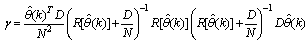 The third method is the K-step ahead predictions [10] where the outputs of the trained network are compared to the unscaled output training data. The K-step ahead predictor follows directly from (8) and for
  and
and , takes the following form:
 | (26) |
where

 The mean value of the K-step ahead prediction error (MVPE) between the predicted output and the actual training data set is computed as follows:
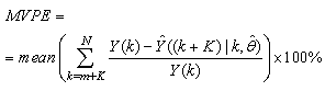 | (27) |
where  corresponds to the unscaled output training data and
  the K-step ahead predictor output.
4. Formulation of the Neural Network–Based Online Prediction Problem for the Influent Characteristics
4.1. Selection of the Manipulated Inputs and Controlled Outputs of the Influent Characteristics Problem
The online determination of the influent characteristics prior to its arrival at the wastewater treatment environment can give information about the control requirements. This idea for predicting the influent characteristics, as illustrated in Fig.4 based on ANN, is by evaluating the influent quality index (IQ), chemical oxygen demand (COD_inf), biochemical oxygen demand (BOD_inf), total Kjeldahl nitrogen (TKN) and the food-to-microoganisms ratio (F_M_R) as predicted outputs using TSS_inf, XS_inf, XI_inf, XBH_inf, XBA_inf, XP_inf, SNH_inf, SND_inf, XND_inf, SS_inf, SI_inf, SO_inf, SNO_inf, SN_inf and Salk_inf as inputs. Based on the COST 624 standards, the expected values for predicted outputs should be for TKN_inf = 10 g.m-3, BOD_inf = 2 g.m-3, COD_inf = 48.2 g.m-3, Influent quality (IQ) = 42000 kg.d-1, ammonia and ammonium nitrogen (SNH_pinf) = 4 g.m-3, total sludge = 18692.5 kg, MLVSS = 1130 g.m-3, TSS = 211.3 g.m-3 and food-to-microorganisms ratio (F:M ratio) = 0.2 mg.BOD/mg. MLVSS. These predicted outputs forms the decision parameters and the starting point for the design of the adaptive self-organizing fuzzy logic controller and its implementation in our next study.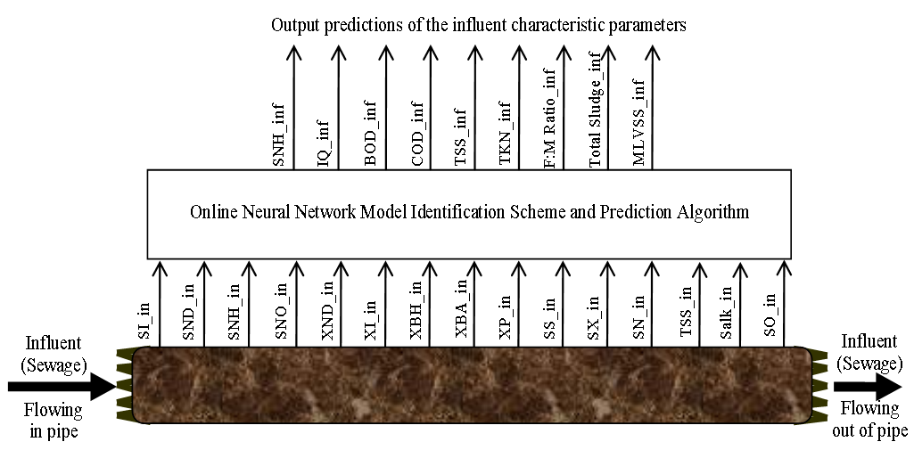 | Figure 4. The proposed scheme for the neural network-based NNAMARX model identification and prediction of the incoming influent characteristics for the AS-WWTP process |
4.2. Formulation of the AS-WWTP Influent Characteristics Model Identification and Prediction Problem
4.2.1. Statement of the AS-WWTP Influent Characteristics Neural Network Model Identification Problem
The activated sludge wastewater treatment plant model defined by the benchmark simulation model no. 1 (BSM1) is described by eight coupled nonlinear differential equations given in Appendix A. The BSM1 model consist of thirteen states defined in Table 1 but they are redefined here for the incoming influent (with I and subscript in and inf for inputs and outputs respectively) as follows: 
 and
and  for the inputs; while


 and
and  are the outputs. Out of thirteen states, only four states are measurable namely:
  (readily biodegradable substrate),
  (active heterotrophic biomass),
  (oxygen) and
  (nitrate and nitrite nitrogen).Thus, from the discussions so far, the measured inputs that influence the behaviour of the influent characteristics of the AS-WWTP process shown in Fig. 5 are:
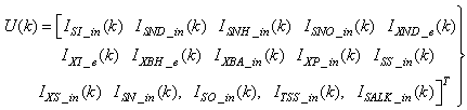 | (28) |
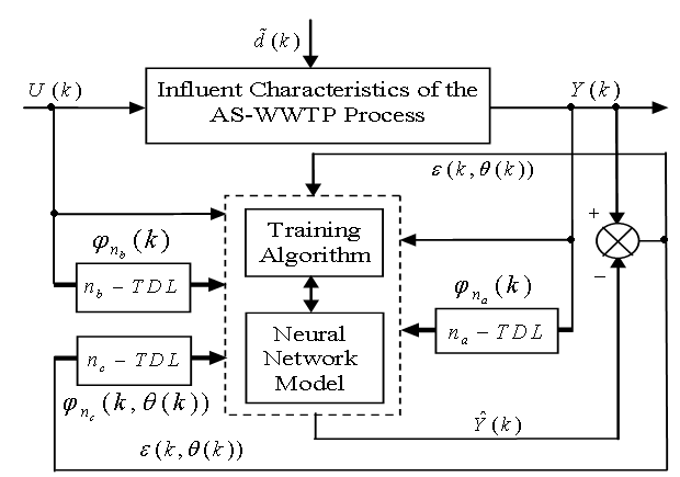 | Figure 5. The neural network model identification scheme for modeling and prediction of the influent (sewage) characteristics based on NNARMAX model structure |
Furthermore, based on the discussions thus far, the output parameters that can be used to determine the influent characteristics of the AS-WWTP are defined here as: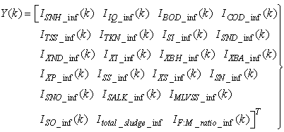 | (29) |
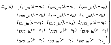
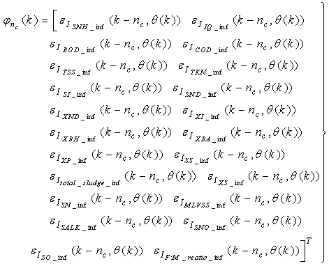
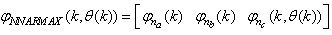
Although, the system is formulated as 15–input 9–output problem, the neural network model identification is a much more complicated multiple–input multiple–output (MIMO) problem since all the fiftteen states must be predicted at each sampling instant in order to compute the parameters that are further used for the prediction of the influent characteristics. Thus, making the total outputs 22 instead of 24 where SNH_inf and TSS_inf have been excluded to avoid repetition. Additional complexity arises from the number of past inputs and outputs in the regression matrix that defines the system. The series-parallel neural network identification scheme used here is shown in Fig. 5 and is based on the NNARMAX model predictor discussed in Section 3. The input vector to the neural network (NN) consists of the regression vectors which are concatenated into 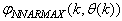 for the NNARMAX model predictor discussed in Section 3 and defined here as follows:
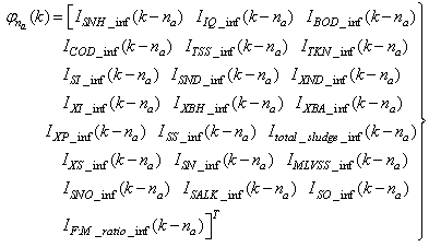 | (30) |
 | (31) |
 | (32) |
 | (33) |
The outputs of the neural network for the AS-WWTP process are the predicted values of the fourteen states together with the nine output parameters that are used to determine the influent characteristics. Thus, resulting in 21 parameters to be predicted at each sampling instant given by: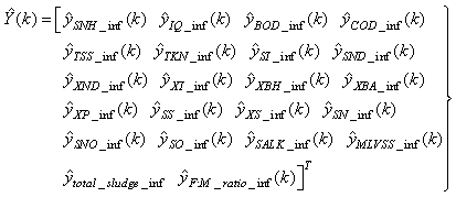 | (34) |
Since disturbances play important roles in the evaluation of controller performances, three influent disturbance data are defined for the three different weather conditions, namely: dry-weather data, rain weather data, and storm weather data. The data for these three influent disturbances are provided by the European COST Actions for evaluating controller performances [4]–[6], [8]. In this study, the dry weather influent data is used in order to measure how well the trained neural network mimic the dynamics of the AS-WWTP process to meet the control requirement specified above. The dry weather data contains two weeks of influent data at 15 minutes sampling interval. Although, disturbances  affecting the AS-WWTP are incorporated into dry-weather data provided by the COST Action Group, additional sinusoidal disturbances with non-smooth nonlinearities are introduced to further investigate the closed-loop performances based on an updated neural network model at each sampling time instants.
4.2.2. Experiment with the BSM1 for AS-WWTP Process Neural Network Training Data Acquisition
For the efficient control of the activated sludge wastewater treatment plant (AS-WWTP) using neural network, a neural network (NN) model of the AS-WWTP process is needed which requires that the NN be trained with dynamic data obtained from the AS-WWTP process. In other to obtain dynamic data for the NN training, the validated and generally accepted COST Actions 624 benchmark simulation model no. 1 (BSM1) is implemented and simulated using MATLAB and Simulink as shown in Fig. 6. The BSM1 process model for the AS-WWTP process is given in Appendix A.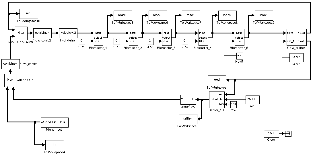 | Figure 6. Open-loop steady-state benchmark simulation model No.1 (BSM1) with constant influent |
A two-step simulation procedure defined in the COST Actions simulation benchmark [4]–[6], [8] is used in this study. The first step is the steady state simulation using the constant influent flow (CONSTINFLUENT) for 150 days as shown and implemented in Fig. 6. Note that each simulation sample period indicated by the “Clock” of the AS-WWTP Simulink model in Fig. 6 corresponds to one day. In the second step, starting from the steady state solution obtained with the CONSTINFLUENT data and using the dry-weather influent weather data (DRYINFLUENT) as inputs, the AS-WWTP process is then simulated for 14 days using the same Simulink model of Fig. 6 but by replacing the CONSTINFLUENT influent data with the DRYINFLUENT influent data. This second simulation generates 1345 dynamic data in which is used for NN training while the 130 first day dry-weather data samples provided by the COST Actions 624 and 682 is used for the trained NN validation.
4.2.3. The Incremental or Online Back-Propagation (INCBP) Algorithm
In order to investigate the performance of the ARLS, the so-called incremental (or online) back-propagation (INCBP) algorithm is used for this purpose. The incremental or online back-propagation (INCBP) algorithm was originally proposed by [13] which has been modified in [7], [8] is used in this paper. The incremental back-propagation (INCBP) algorithm is easily derived by setting the covariance matrix  on the left hand side of (20) in Section 3.3.1under the formulation of the ARLS algorithm; that is:
 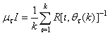 | (35) |
where  is the step size and
  is an identity matrix of appropriate dimension. Next, the basic back-propagation given from [10] as:
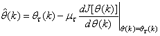 | (36) |
is used to update the algorithm in (35). Finally, all that is required is to specify a suitable step size  and carry out the recursive computation of the gradient given by (36).
4.2.4. Scaling the Training Data and Rescaling the Trained Network that Models the AS-WWTP Process
Due to the fact the input and outputs of a process may, in general, have different physical units and magnitudes; the scaling of all signals to the same variance is necessary to prevent signals of largest magnitudes from dominating the identified model. Moreover, scaling improves the numerical robustness of the training algorithm, leads to faster convergence and gives better models. The training data are scaled to unit variance using their mean values and standard deviations according to the following equations [7], [8]: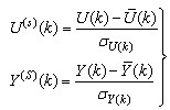 | (37) |
where  and
and  are the mean and standard deviation of the input and output training data pair; and
  and
and  are the scaled inputs and outputs respectively. Also, after the network training, the joint weights are rescaled according to the expression
 | (38) |
so that the trained network can work with other unscaled validation data and test data not used for training. However, for notational convenience,  and
and  shall be used.
4.2.5. Training the Neural Network that Models the Biological Reactors of the AS-WWTP Process
The NN input vector to the neural network (NN) is the NNARMAX model regression vector  defined by (33). The input
  , that is the initial error estimates
  given by (32), is not known in advance and it is initialized to small positive random matrix of dimension
  by
by . The outputs of the NN are the predicted values of
  given by (34).For assessing the convergence performance, the network was trained for
  epochs (number of iterations) with the following selected parameters:
 (NNARMAX),
 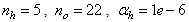 and
and  . The details of these parameters are discussed in Section 3; where
  and
and  are the number of inputs and outputs of the system,
  and
and  are the orders of the regressors in terms of the past values,
  is the total number of regressors (that is, the total number of inputs to the network),
  and
and  are the number of hidden and output layers neurons, and
  and
and  are the hidden and output layers weight decay terms. The four design parameters for adaptive recursive least squares (ARLS) algorithm defined in (22) are selected to be: α=0.5, β=5e-3,
  =1e-5 and π=0.99 resulting to γ=0.0101. The initial values for ēmin and ēmax in (23) are equal to 0.0102 and 1.0106e+3 respectively and were evaluated using (23). Thus, the ratio of ēmin/ēmax from (23) is 9.9018e+4 which imply that the parameters are well selected. Also,
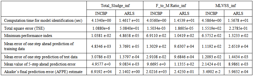
  is selected to initialize the INCBP algorithm given in (36).The 1345 dry-weather training data is first scaled using equation (37) and the network is trained for τ = 50 epochs using the proposed adaptive recursive least squares (ARLS) and the incremental back-propagation (INCBP) algorithms proposed in Sections 3.3 and 4.2.3. After network training, the trained network is again rescaled respectively according to (38), so that the resulting network can work or be used with unscaled AS-WWTP data. Although, the convergence curves of the INCBP and the ARLS algorithms for 50 epochs each are not shown but the minimum performance indexes for both algorithms are given in the third rows of Tables 4(a), (b) and (c). As one can observe from these Tables, the ARLS has smaller performance index when compared to the INCBP which is an indication of good convergence property of the ARLS at the expense of higher computation time when compared the small computation time used by the INCBP for 50 epochs as evident in the first rows of Tables 4(a), (b) and (c).The total square error (TSE) discussed in subsection 3.1, for the network trained with the INCBP and the ARLS algorithms are given in the second rows of Table 4(a), (b) and (c). Again, the ARLS algorithm also has smaller mean square errors and minimum performance indices when compared to the INCBP algorithm. The small values of the total square error (TSE) and the minimum performance indices indicate that ARLS performs better than the INCBP for the same number of iterations (epochs). These small errors suggest that the ARLS model approximates better the AS-WWTP process giving smaller errors than the INCBP model.
4.3. Validation of the Trained NNARMAX Model for the Prediction of the Influent Characteristics for the AS-WWTP Process
According to the discussion on network validation in Section 3.4, a trained network can be used to model a process once it is validated and accepted, that is, the network demonstrates its ability to predict correctly both the data that were used for its training and other data that were not used during training. The network trained by the INCBP and the proposed ARLS algorithms has been validated with three different methods by the use of scaled and unscaled training data as well as with the 130 dry-weather data reserved for the validation of the trained network for the AS-WWTP process.
4.3.1. Validation by the One-Step Ahead Predictions Simulation
In the one-step ahead prediction method, the errors obtained from one-step ahead output predictions of the trained network are assessed. In Fig. 7(a)–(i) the graphs for the one-step ahead predictions of the scaled training data (blue -) against the trained network output predictions (red --*) using the neural network models trained by INCBP and ARLS algorithms respectively are shown for 50 epochs.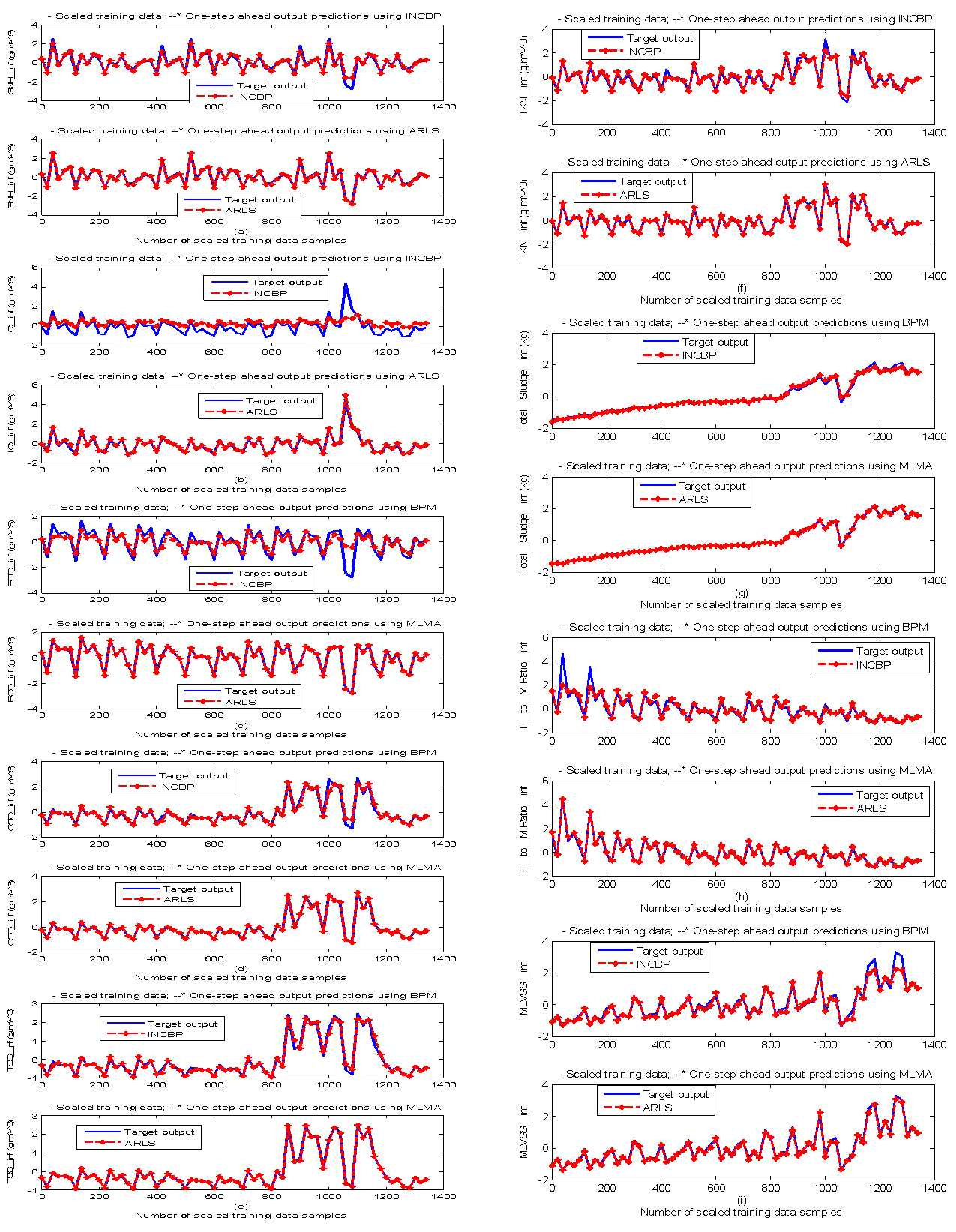 | Figure 7(a). Comparison of the one-step ahead prediction of scaled training data by INCBP and ARLS: (a) SNH_inf, (b) IQ_inf, (c) BOD_inf, (d) COD_inf, (e) TSS_inf, (f) TKN_inf, (g) Total_Sludge_inf, (h) F_to_M Ratio_inf, (i) MLVSS_inf |
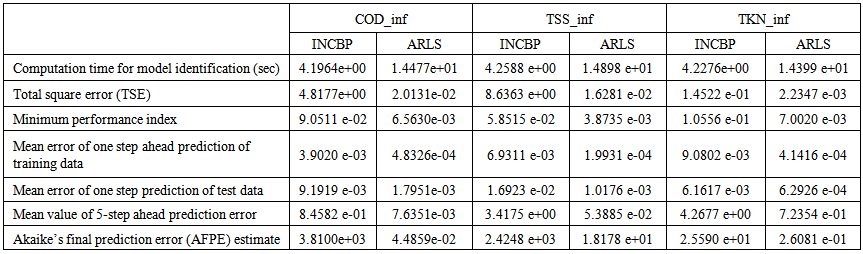
The mean value of the one-step ahead prediction errors are given in the fourth rows of Table 4(a), (b) and (c) respectively. It can be seen in the figures that the network predictions of the training data closely match the original training data. Although, the scaled training data prediction errors by both algorithms are small, the ARLS algorithm appears to have a much smaller error when compared to the INCBP algorithm as shown in the fourth rows of Table 4(a), (b) and (c). These small one-step ahead prediction errors are indications that the networks trained using the ARLS captures and approximate the nonlinear dynamics of the five reactors of the AS-WWTP process to a high degree of accuracy. This is further justified by the small mean values of the TSE obtained for the networks trained using the proposed ARLS algorithms for the process as shown in the second rows of Table 4(a), (b) and (c).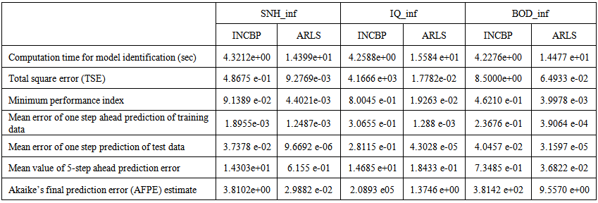 | Table 4(a). Influent characteristics and the influent constrained parameter predictions |
 | Table 4(b). Influent characteristics and the influent constrained parameter predictions |
 | Table 4(c). Influent characteristics and the influent constrained parameter predictions |
Furthermore, the suitability of the INCBP and the proposed ARLS algorithms for neural network model identification for use in the real AS-WWTP industrial environment is investigated by validating the trained network with the 130 unscaled dynamic data obtained for dry-weather as provided by the COST Action Group. Graphs of the trained network predictions (red --*) of the validation (test) data with the actual validation data (blue -) using the INCBP and the proposed ARLS algorithms are shown in Fig. 8(a)–(i) for the five reactors of the AS-WWTP process based on the selected process parameters. The almost identical prediction of these data proves the effectiveness of the proposed approaches. The prediction accuracies of the unscaled test data by the networks trained using the INCBP and the proposed ARLS algorithm evaluated by the computed mean prediction errors shown in the fifth rows of Table 4(a), (b) and (c). Again, one can observe that although the validation data prediction errors obtained by both algorithms are small, the validation data predictions errors obtained with the model trained by the proposed ARLS algorithm appears much smaller when compared to those obtained by the model trained using the INCBP algorithm. These predictions of the unscaled validation data given in Fig. 8(a)–(i) as well as the mean value of the one step ahead validation (test) prediction errors in the fifth rows of Tables 4(a), (b) and (c) verifies the neural network ability to model accurately the dynamics of the five reactors of the AS-WWTP process based on the dry-weather influent data using the proposed ARLS training algorithm.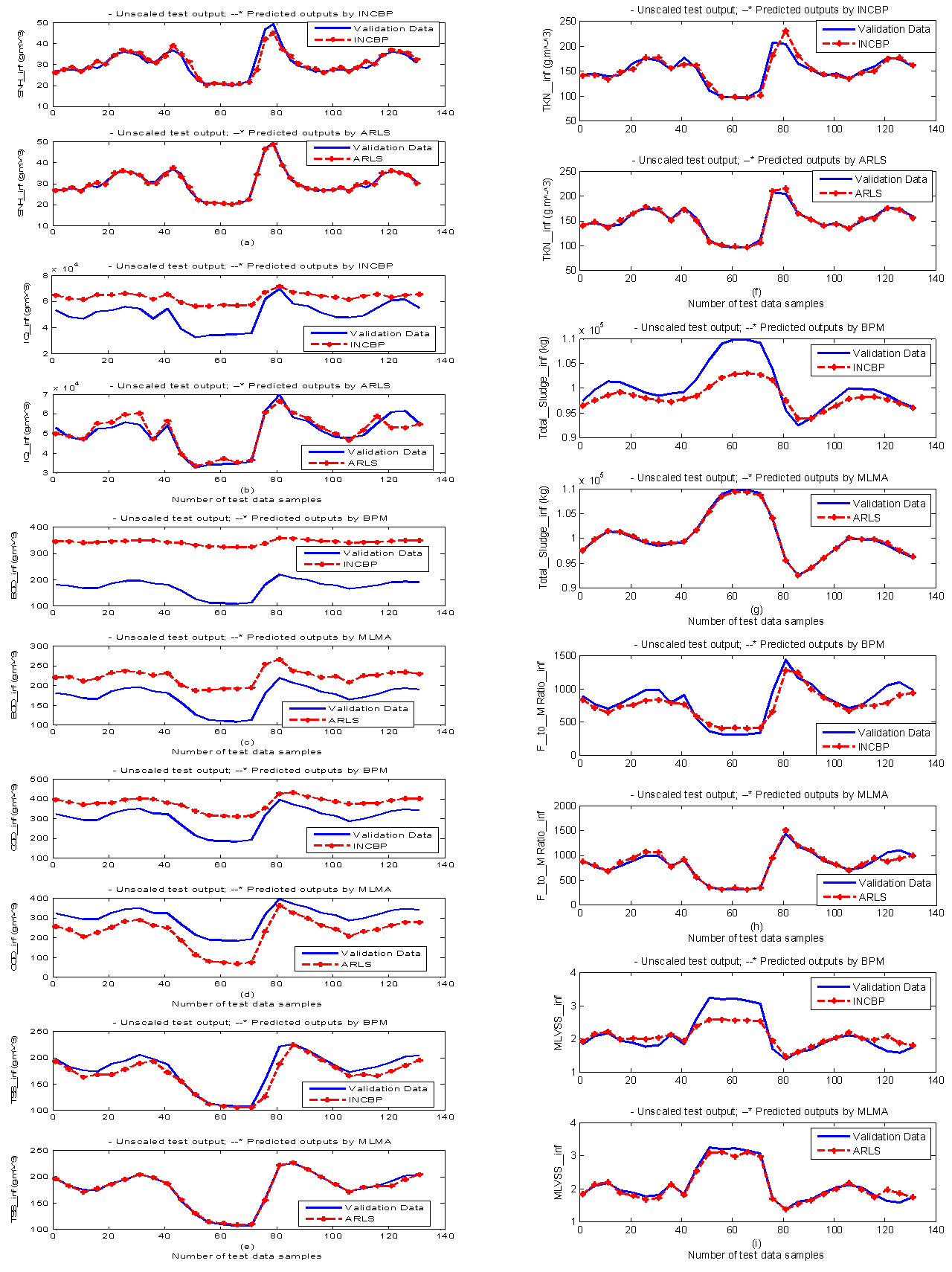 | Figure 8(a). Comparison of the one-step ahead prediction of unscaled validation data by INCBP and ARLS: (a) SNH_inf, (b) IQ_inf, (c) BOD_inf, (d) COD_inf, (e) TSS_inf, (f) TKN_inf, (g) Total_Sludge_inf, (h) F_to_M Ratio_inf, (i) MLVSS_inf |
4.3.2. K–Step Ahead Prediction Simulations for the AS-WWTP Process
The results of the K-step ahead output predictions (red --*) using the K-step ahead prediction validation method discussed in Section 3.4 for 5-step ahead output predictions (K = 5) compared with the unscaled training data (blue -) are shown in Fig. 9(a) to Fig. 9(i) for the networks trained using the INCBP and the proposed ARLS. Again, the value K = 5 is chosen since it is a typical value used in most model predictive control (MPC) applications. The comparison of the 5-step ahead output predictions performance by the network trained using the INCBP and the proposed ARLS algorithms indicate the superiority of the proposed ARLS over the so-called INCBP algorithm.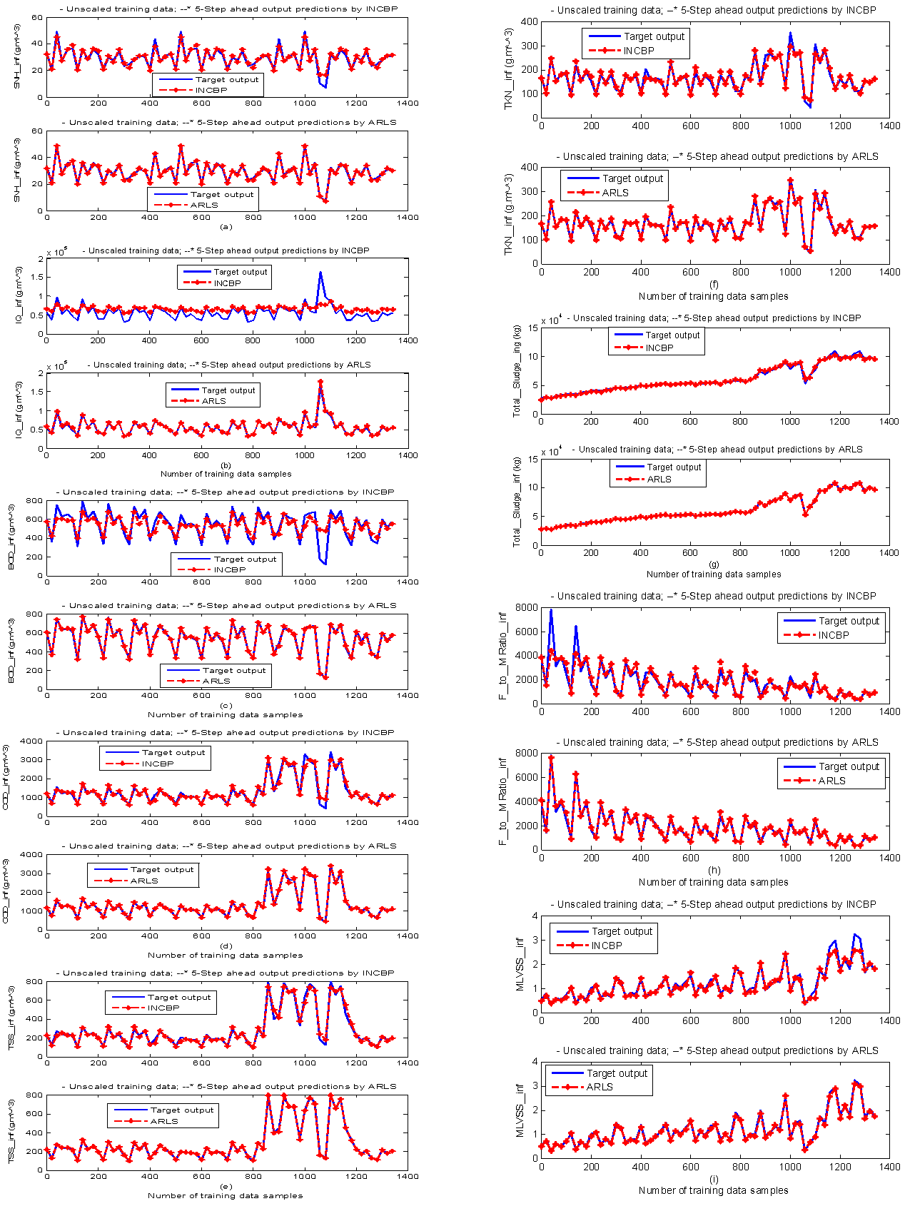 | Figure 9(a). Comparison of the five-step ahead prediction of unscaled training data by INCBP and ARLS: (a) SNH_inf, (b) IQ_inf, (c) BOD_inf, (d) COD_inf, (e) TSS_inf, (f) TKN_inf, (g) Total_Sludge_inf, (h) F_to_M Ratio_inf, (i) MLVSS_inf |
The computation of the mean value of the K-step ahead prediction error (MVPE) using (27) is given in the sixth rows of Tables 4(a), (b) and (c) by the network trained using INCBP and the proposed ARLS algorithms respectively. The small mean values of the 5-step ahead prediction error (MVPE) are indications that the trained network approximates the dynamics of the five reactors of the AS-WWTP process to a high degree of accuracy with the networks of both algorithms but with the network based on the ARLS algorithm giving much smaller distant prediction errors.
4.3.3. Akaike’s Final Prediction Error (AFPE) Estimates for the AS-WWTP Process
The implementation of the AFPE algorithm discussed in Section 3.4 and defined by (25) for the regularized criterion for the network trained using the INCBP and the proposed ARLS algorithms with multiple weight decay gives their respective AFPE estimates which are defined in the seventh rows of Tables 4(a), (b) and (c) respectively. These relatively small values of the AFPE estimate indicate that the trained networks capture the underlying dynamics of the aerobic reactor of the AS-WWTP and that the network is not over-trained [9]. This in turn implies that optimal network parameters have been selected including the weight decay parameters. Again, the results of the AFPE estimates computed for the networks trained using the proposed ARLS algorithm are much smaller when compared to those obtained using INCBP algorithm.
4.3.4. Influent Characteristics Prediction Based on the CST Action Constrained Parameters for the Influent
In order to predict the influent characteristics of the incoming influent (sewage), the Simulink model of the AS-WWTP process shown in Fig. 6 has been simulated in closed-loop with +30% disturbances about the nominal values of all the input parameters distributed over 200 random samples in 200 simulations. However, due to space economy, on 10 simulations (Sim) results at an interval of 20 samples are shown in Table 5. Note that in Table 5, the last column shows the nominal values as published by COST Actions 624 and 628 [4]–[6].It can be seen from Table 5 that both the INCBP and the ARLS algorithms gives appreciable predictions of all the influent constrained parameters. A close study of Table 5 further reveals that the better prediction results are obtained using the NN models trained with ARLS. For clarity, the results of Table 5 is plot as shown in Fig. 10 where the prediction performances by the models based on INCBP and ARLS are compared to the COST standards. As it can be seen in Fig. 10, (a), (b), (c), (d) and (f) are completely out of phase when compared to COST standard for our simulation studies. However, the predictions in (e), (g), (h) and (i) fluctuates around and are within the ranges of the COST standards except for the MLVSS_inf in (i) due to INCBP.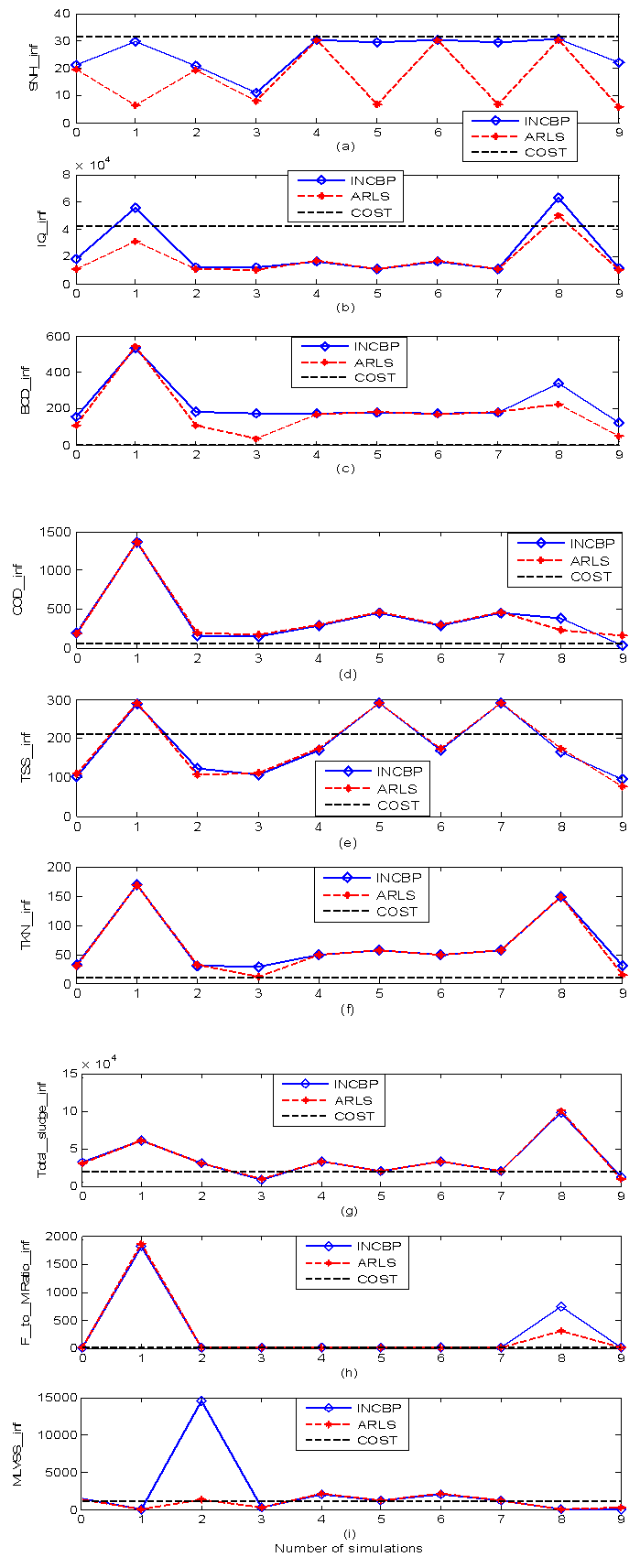 | Figure 10. Comparison of the constrained parameter predictions by models trained using INCBP and ARLS with the true COST Actions standards: (a) SNH_inf, (b) IQ_inf, (c) BOD_inf, (d) COD_inf, (e) TSS_inf, (f) TKN_inf, (g) Total_Sludge_inf, (h) F_to_M Ratio_inf, (i) MLVSS_inf |
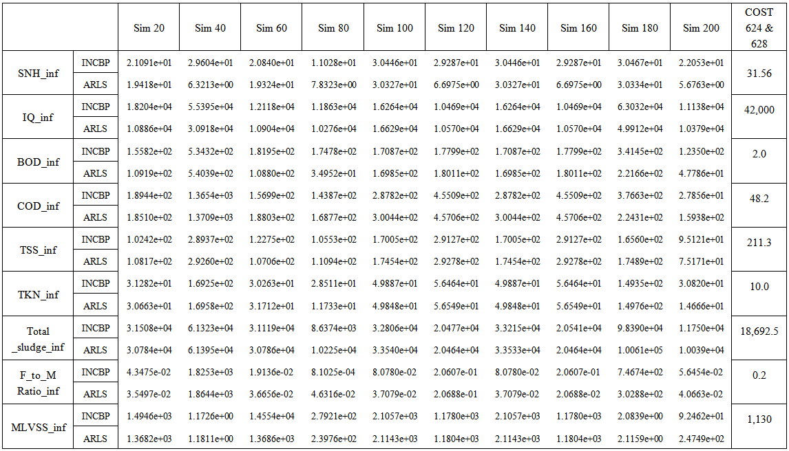 | Table 5. Mean values of the constrained parameters for the prediction of the influent characteristics in 10 simulation studies |
It is obvious that the incoming influent in the first three simulations (i.e. 0, 1 and 2) is of high toxic content and may be discarded while the incoming influent in the last three simulations (i.e. 7, 8 and 9) may be pretreated before passing it to the WWTP. The incoming influent from the third simulation up the third before the last (i.e. 2, 3, 4, 5, 6 and 7) can channeled directly to the WWTP.
5. Conclusions
This paper presents a novel problem formulation for the prediction of influent characteristics together with the formulation of advanced online nonlinear adaptive recursive least squares (ARLS) model identification algorithm based on artificial neural networks for the nonlinear model identification and performance parameter prediction for AS-ASWWTP process management. In order to investigate the performance of the proposed ARLS algorithm, the incremental backpropagation (INCBP), which is also an online algorithm, is implemented and compared with proposed ARLS. The results from the application of these algorithms to the modelling and prediction of the influent characteristics as well as the validation results show that the neural network-based ARLS outperforms the INCBP algorithm with much smaller predictions error and good tracking and prediction abilities with an appreciable degree of accuracy. It is concluded that the proposed ARLS model identification algorithm can be used for the AS-ASWWTP process in an industrial environment.From the view point of the authors, the nonlinear modeling and adaptive control of the AS-WWTP process is better formulated as a five-stage multivariable modeling and control problem with tight constraints because of its nonlinear and structural complexities. Thus, as a first step, the online prediction of the incoming influent (sewage) characteristics has been considered. The next stage is on the nonlinear modeling of the biological reactors followed by the nonlinear modeling of the secondary settler and clarifier. The fourth stage is on the development and implementation of an intelligent self-organizing fuzzy logic decision controller (SOFLDC) for the complete AS-WWTP process. The fifth stage is on the development of a nonlinear adaptive model-based predictive control (NAMBPC) algorithm for the adaptive control of the complete AS-WWTP by manipulating the pumps based on some decision parameters.The next aspect of the work is on the dynamic modelling and nonlinear model identification of the multivariable NNARMAX model of the secondary settler and the clarifier as well as effluent tank to complete the modelling of the AS-WWTP process.
Appendix
Appendix A: AS-WWTP Process Model
As mentioned in above, the BSM1 model involves eight different chemical reactions  incorporating thirteen different components [4]–[6], [8]. These components are classified into soluble components
  and particulate components
 . The nomenclatures and parameter definitions used for describing the AS-WWTP in this work are given in Table 1. The Moreover, four fundamental processes are considered: the growth and decay of biomass (heterotrophic and autotrophic), ammonification of organic nitrogen and the hydrolysis of particulate organics. The typical schematic of the AS-WWTP is shown in Fig. 1.
The eight basic processes that are used to describe the biological behaviour of the AS-WWTP process are: : Aerobic growth of heterotrophs
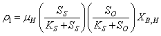 | (A.1) |
 : Anoic growth of heterotrophs
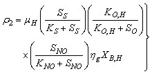 | (A.2) |
 : Aerobic growth of autotrophs
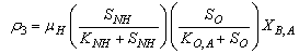 | (A.3) |
 : Decay of heterotrophs
 | (A.4) |
 : Decay of autotrophs
 | (A.5) |
 : Ammonification of soluble organic nitrogen
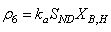 | (A.6) |
 : Hydrolysis of entrapped organics
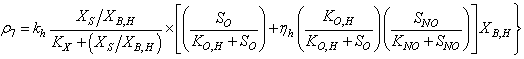 | (A.7) |
 : Hydrolysis of entrapped organic nitrogen
 | (A.8) |
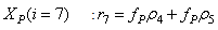
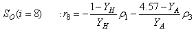
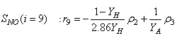
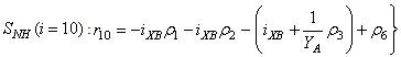
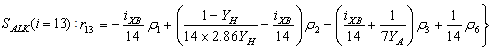
The observed thirteen conversion rates  result from combinations of basic processes (A.1) to (A.8) as follows:
 | (A.9) |
 | (A.10) |
 | (A.11) |
 | (A.12) |
 | (A.13) |
 | (A.14) |
 | (A.15) |
 | (A.16) |
 | (A.17) |
 | (A.18) |
 | (A.19) |
 | (A.20) |
 | (A.21) |
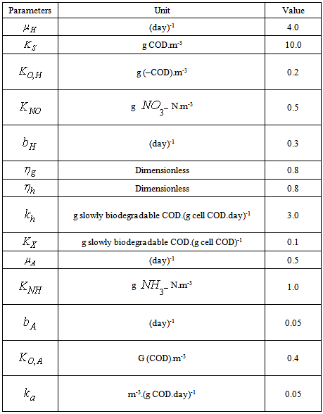
The biological parameter values used in the BSM1 correspond approximately to a temperature of 15°C. The stiochiometric parameters are listed in Table A.1 and the kinetic parameters are listed in Table A.2.Table A.1. Stiochiometric parameters with their units and values
 |
| |
|
Table A.2. Kinetic parameters with their units and values
 |
| |
|
Appendix B: Criteria for Evaluating and Assessing the Performances of the AS-WWTP Control
Appendix B.1: Influent Quality (IQ)
As a check on the IQ calculation, an influent quality index (IQ) can be calculated by applying the above equations to the influent file but the BOD coefficient must be changed from 0.25 to 0.65. It is defined as: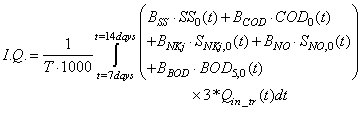 | (B.1) |
where the composition variables are calculated as follows: | (B.2) |
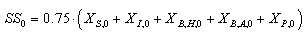 | (B.3) |
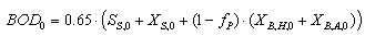 | (B.4) |
 | (B.5) |
and the  above are weighting factors for the different types of pollution to convert them into pollution units
  and were chosen to reflect these calculated fractions as follows:
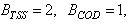

 and
and  .
.
Appendix B.2: The Sludge Production to be Disposed
This is the sludge production,  is calculated from the total solid flow from wastage and solid accumulated in the system over the period of time considered
  for each weather file). The amount of solids in the system at time t is given by:
  | (B.6) |
where  is the amount of solids in the reactor given by:
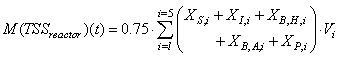 | (B.7) |
 is the amount of solids in the settler given by:
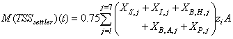 | (B.8) |
 the change in system sludge mass from the end of day 7 to the end of day 14 given by:
 and
and  the amount of waste sludge is given by:
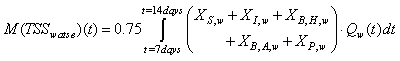 | (B.9) |
So that the total sludge to be disposed becomes: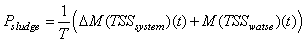 | (B.10) |
Appendix B.3: The Total Sludge Production 
The total sludge production takes into account the sludge to be disposed and the sludge lost to the weir and is calculated as follows: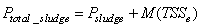 | (B.11) |
where 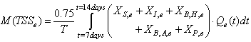
References
| [1] | M. Henze, P. Harremoës, J. Jansen and E. Arvin, “Wastewater Treatment,” Biological and Chemical Processes, 2nd ed., Berlin: Springer Verlag, 1996. |
| [2] | E. Arden and W. T. Lockett, “Experiments on the oxidation of sewage without the aid of filters”, J. Soc. Chem. Ind., vol. 33, pp. 523 – 539. |
| [3] | F.R. Spellman, Handbook of Water and Wastewater Treatment Plant Operations. Boca Raton, Florida: CRC Press LLC, 2003. |
| [4] | J.B. Coop. (2000, Sept.). The COST Simulation Benchmark: Description and Simulation Manual (a product of COST Actions 624 & 628). [Online]. Available:http://www.ensic.inpl-nancy.fr/COSTWWTP/. |
| [5] | Working Groups of COST Actions 632 and 624. (2000, Sept.). IWA Task Group on Benchmarking of Control Strategies for WWTPs. [Online]. Available:http://www.ensic.inpl-nancy.fr/benchmarkWWTP/Bsm1/Benchmark1.htm. |
| [6] | Working Groups of COST Actions 632 and 624. (Apr., 2008). IWA Task Group on Benchmarking of Control Strategies for WWTPs:http://www.ensic.inplnancy.fr/benchmarkWWTP/Bsm1/Benchmark1.htm. |
| [7] | V. A. Akpan and G. D. Hassapis, “Training dynamic feedforward neural networks for online nonlinear model identification and control applications”. International Reviews of Automatic Control: Theory & Applications, vol. 4, no. 3, pp. 335 – 350, 2011. |
| [8] | V. A. Akpan (Jul., 2011): Development of new model adaptive predictive control algorithms and their implementation on real-time embedded systems, Ph.D. Dissertation, 517 pages. [Online] Available:http://invenio.lib.auth.gr/record/127274/files/GRI-2011-7292.pdf. |
| [9] | A. Iratni, R. Katebi, R. Vilanova and M. Mostefai, “On estimation of unknown state variables in wastewater systems”, In the Proceedings of the 14th IEEE International Conference on Emerging Technologies and Factory Automation (ETFA’2009), Palma de Mallorca, Spain, 22 – 26 Sept., 2009, pp. 1 – 8. |
| [10] | L. Lung, System Identification: Theory for the User. 2nd ed. Prentice-Hall, 1999. |
| [11] | V. A. Akpan and G. D. Hassapis, “Nonlinear model identification and adaptive model predictive control using neural networks”, ISA Transactions, vol. 50, no. 2, pp. 177 – 194, 2011. |
| [12] | J. Sjöberg and L. Ljung, Overtraining, regularization, and searching for minimum in neural networks, International Journal of Control, vol. 62: 1391-1408, 1995. |
| [13] | J. Hertz, A. Krough and R. G. Palmer, “An Introduction to the Theory of Neural Computation”, Lecture Notes, vol. 1, Redwood City, California: Addison-Wesley, 1991. |
 Abstract
 Reference
 Full-Text PDF
 Full-text HTML