-
Paper Information
- Previous Paper
- Paper Submission
-
Journal Information
- About This Journal
- Editorial Board
- Current Issue
- Archive
- Author Guidelines
- Contact Us
American Journal of Intelligent Systems
p-ISSN: 2165-8978 e-ISSN: 2165-8994
2014; 4(3): 77-106
doi:10.5923/j.ajis.20140403.02
Multivariable NNARMAX Model Identification of an AS-WWTP Using ARLS: Part 2 – Dynamic Modeling of the Secondary Settler and Clarifier
 Abstract
 Reference
 Full-Text PDF
 Full-text HTML
Vincent A. Akpan1, Reginald A. O. Osakwe2
1Department of Physics Electronics, The Federal University of Technology, P.M.B. 704, Akure, Ondo State, Nigeria
2Department of Physics, The Federal University of Petroleum Resources, P.M.B. 1221, Effurun, Delta State, Nigeria
Correspondence to: Vincent A. Akpan, Department of Physics Electronics, The Federal University of Technology, P.M.B. 704, Akure, Ondo State, Nigeria.
| Email: |  |
Copyright © 2014 Scientific & Academic Publishing. All Rights Reserved.
This paper presents the formulation and application of an online adaptive recursive least squares (ARLS) algorithm to the nonlinear model identification of the secondary settler/clarifier and the effluent tank of an activated sludge wastewater treatment (AS-WWTP). The performance of the proposed ARLS algorithm is compared with the so-called incremental backpropagation (INCBP) which is also an online identification. These algorithms are validated by one-step and five-step ahead prediction methods. The performance of the two algorithms is also assessed by using the Akaike’s method to estimate the final prediction error (AFPE) of the regularized criterion. The validation results show the superior performance of the proposed ARLS algorithm in terms of much smaller prediction errors when compared to the INCBP algorithm.
Keywords: Activated sludge wastewater treatment plant (AS-WWTP), Adaptive recursive least squares (ARLS), Artificial neural network (ANN), Benchmark simulation model No. 1 (BSM #1), Biological reactors, Effluent tank, incremental backpropagation (INCBP), Nonlinear model identification, Nonlinear neural network autoregressive moving average with exogenous input (NNARMAX) model, Secondary settler and clarifier
Cite this paper: Vincent A. Akpan, Reginald A. O. Osakwe, Multivariable NNARMAX Model Identification of an AS-WWTP Using ARLS: Part 2 – Dynamic Modeling of the Secondary Settler and Clarifier, American Journal of Intelligent Systems, Vol. 4 No. 3, 2014, pp. 77-106. doi: 10.5923/j.ajis.20140403.02.
Article Outline
1. Introduction
- Biological approach is the most widely used industrial technique in the wastewater treatment engineering community. The activated sludge process [1-5] is the most widely used system for biological wastewater treatment. Traditionally, activated sludge process (ASP) involve an anaerobic (anoxic) followed by an aerobic zone and a settler from which the major part of the biomass is recycled to the anoxic basin and this prevents washout of the process by decoupling the sludge retention time (SRT) from the hydraulic retention time (HRT). Activated sludge wastewater treatment plants (ASWWTP) are built to remove organic mater from wastewater where a bacterial biomass suspension (the activated sludge) is responsible for the removal of pollutants. Depending on the design and specific application, ASWWTP can achieve biological nitrogen removal, biological phosphorus removal and removal of organic carbon substances as well as the amount of dissolved oxygen [6]. Generally, an ASWWTP can generally be regarded as a complex system due to its highly nonlinear dynamics, large uncertainty, multiple time scales in the internal processes as well as its multivariable structure [7-10]. A widely accepted biodegradation model is the activated sludge model no. 1 (ASM #1) which incorporate the basic biotransformation processes of an ASP [1, 2, 7].Two of the critical points affecting classical biological reactors are controlling the sludge height in the secondary settler and the secondary settler efficiency, where the mixed liquor from the biological reactors is settled in order to obtain a clarified effluent prior to final discharge. The secondary settler parameters involved in the settling phase and those that highly affect the pollution removal process efficiency have been exploited by some authors [11-13]. A methodology to control the sludge blanket by measuring simple on-line (influent flow) parameters and off-line (a daily measured sludge volumetric index, SVI) parameters and manipulating the RAS recycle flow has been reported [14]. In the work of [14], the ability of fuzzy logic to integrate human knowledge was exploited to develop a fuzzy controller to maintain the secondary settler under stable conditions.Biological nutrient removal (BNR) systems are reliable and effective in removing nitrogen and phosphorus. The process is based upon the principle that under specific conditions, microorganisms will remove more phosphorus and nitrogen than is required for biological activity. However, several research papers have been published [8, 9], [15-19] concerning the BNR but the performance still depends on the biological activity and the process employed and it is an open intensive research field with emphasis on the effluent quality and operational cost.The mixture of activated sludge and wastewater in the aeration tank together with the mixed liquor flows to a secondary settler and clarifier where the activated sludge is allowed to settle. The activated sludge is constantly growing and more is produced than can be returned for use in the aeration basin. Some of this sludge must be wasted to a sludge handling system for treatment and disposal (solids) or reuse (bio-solids). The volume of sludge returned to the aeration basins is normally 40 to 60% of the wastewater flow while the rest is wasted (solids) or reuse (bio-solids).A number of factors affect the performance of the activated sludge system [20, 21]. These include the following: (i) temperature, (ii) return rates, (iii) amount of oxygen available, (iv) amount of organic matter available, (v) pH, (vi) waste rates, (vii) aeration time and (viii) wastewater toxicity. To obtain the desired level of performance in an activated sludge system, a proper balance must be maintained between the amount of food (organic matter), organisms (activated sludge), and dissolved oxygen (DO). The majority of problems with the activated sludge process result from an imbalance between these three items. The actual operation of an activated-sludge system is regulated by three factors: 1) the quantity of air supplied to the aeration tank; 2) the rate of activated-sludge recirculation; and 3) the amount of excess sludge withdrawn form the system. Sludge wasting is an important operational practice because it allows the establishment of the desired concentration of mixed liquor soluble solids (MLSS), food to microorganisms ratio (F:M ratio), and the sludge age. The algorithm for computing these parameters are given in Appendices A, B and C. It should be mentioned here that air requirements in an activated sludge basin are governed by: 1) BOD loading and the desired removal effluent, 2) volatile suspended solids concentration in the aerator, and 3) suspended solids concentration of the primary effluent (see Appendices A, B and C for details).The aim of the paper is on the efficient modeling of a multivariable nonlinear neural network autoregressive moving average with exogenous input (NNARMAX) model that will capture the nonlinear dynamics of an AS-WWTP, trained with an online adaptive recursive least squares (ARLS) [22], for the purpose of developing an efficient nonlinear adaptive controller for the efficient control of the AS-WWTP process. Due to the multivariable nature of the AS-WWTP, the first paper (Part 1) considered the modeling of the five biological reactors including the influent tank [22] while the current paper (Part 2) is devoted to the modeling of the secondary settler and clarifier. The paper is organized into six sections as follows. Section 2 presents the AS-WWTP process description while Section 3 highlights the operational considerations of the secondary settler and clarifier of the AS-WWTP process. Section 4 is devoted to the formulation of the neural network-based adaptive recursive least squares (ARLS) for model identification. Section 5 presents the neural network-based problem formulation for the secondary settler and the clarifier sections of the AS-WWTP process together with the simulation results and their discussion. The paper concludes in Section 6 with highlights on some major contributions in this paper with subsequent and future directions.
2. The AS-WWTP Process Description
- Activated sludge wastewater treatment plants (WWTPs) are large complex nonlinear multivariable systems, subject to large disturbances, where different physical and biological phenomena take place. Many control strategies have been proposed for wastewater treatment plants but their evaluation and comparison are difficult [1-4]. This is partly due to the variability of the influent, the complexity of the physical and biochemical phenomena, and the large range of time constants (from a few minutes to several days) inherent in the activated sludge process. Additional complication in the evaluation is the lack of standard evaluation criteria.With the tight effluent requirements defined by the European Union and to increase the acceptability of the results from wastewater treatment analysis, the generally accepted COST Actions 624 and 682 benchmark simulation model no. 1 (BSM1) model [1-4] is considered. The BSM1 model uses eight basic different processes to describe the biological behaviour of the AS-WWTP processes. The combinations of the eight basic processes results in thirteen different observed conversion rates as described in [1-4], [22, 23]. These components are classified into soluble components
 and particulate components
  . The nomenclatures and parameter definitions used for describing the AS-WWTP in this work are given in Table 1. Moreover, four fundamental processes are considered: the growth and decay of biomass (heterotrophic and autotrophic), ammonification of organic nitrogen and the hydrolysis of particulate organics.
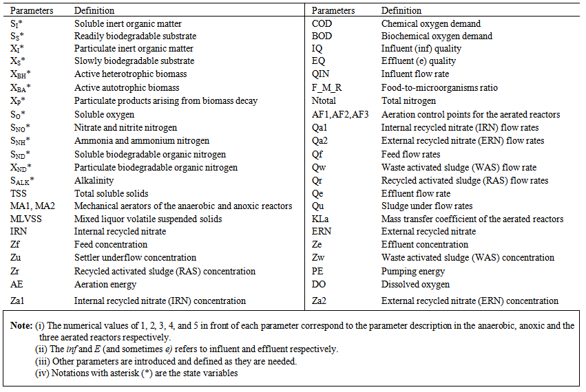 | Table 1. The AS-WWTP Nomenclatures and Parameter Definitions |
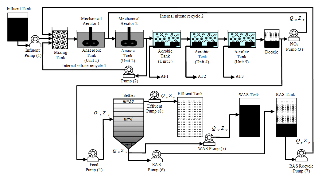 | Figure 1. The schematic of the AS-WWTP process |
3. The Operational Considerations of the Secondary Settler and Clarifier and Effluent Tank of the AS-WWTP
- The activated sludge process generally requires more sampling and testing to maintain adequate process control than any of the other unit processes in the wastewater treatment system. During periods of operational problems, both the parameters tested and the frequency of testing may increase substantially. Process control testing may include the following [20, 21]: 1) settleability testing to determine the settled sludge volume; 2) suspended solids testing to determine influent and MLSS; 3) RAS solids and WAS concentrations; 4) determination of the volatile content of the mixed liquor suspended solids; 5) DO and pH of the aeration tank; 6) BOD and COD of the aeration tank influent and process effluent; and 7) microscopic evaluation of the activated sludge to determine the predominant organism. To maintain the working organisms in the activated sludge process, it is necessary to ensure that a suitable environment is maintained by being aware of the many factors influencing the process and by monitoring them repeatedly. Control, in this case, can be defined as maintaining the proper solids (floc mass) concentration in the aerator for the incoming wastewater flow by adjusting the returned and waste activated sludge pumping rates and regulating the oxygen supply to maintain a satisfactory level of DO in the process.Monitoring alkalinity in the aeration tank is essential to the control of the process. Insufficient alkalinity will reduce organism activity and may result in low effluent pH and, in some cases, extremely high chlorine demand in the disinfection process. However, the pH should also be monitored as part of the routine process control-testing schedule. Processes undergoing nitrification may show a significant decrease in effluent pH. Industrial waste discharges, septic wastes, or significant amounts of storm-water flows may produce wide variations in pH. Finally, because temperature directly affects the activity of the microorganisms, accurate monitoring of temperature can be helpful in identifying the causes of significant changes in organization populations or process performance.The activated sludge process is an aerobic process that requires some DO be present at all times. The amount of oxygen required is dependent on the influent food (BOD), the activity of the activated sludge, and the degree of treatment desired. The mixed liquor suspended solids (MLSS), mixed liquor volatile suspended solids (MLVSS), and mixed liquor total suspended solids (MLTSS) needs to be determined and monitored, by adjusting the MLSS and MLVSS by increasing or decreasing the waste sludge rates. The MLSS or MLVSS can be used to represent the activated sludge or microorganisms present in the process. Process control calculations, such as sludge age and sludge volume index (SVI), cannot be calculated unless the MLSS is determined. The MLTSS is an important activated sludge control parameter. To increase the MLTSS, for example, the operator must decrease the waste rate or increase the mean cell residence time (MCRT). The MCRT must be decreased to prevent the MLTSS from changing when the number of aeration tanks in service is reduced.The separation of solids and liquid in the secondary clarifier results in a blanket of solids. If solids are not removed from the clarifier at the same rate they enter, the blanket will increase in depth. If this occurs, the solids may carry over into the process effluent. The sludge blanket depth may be affected by other conditions, such as temperature variation, toxic wastes, or sludge bulking. The best sludge blanket depth is dependent upon such factors as hydraulic load, clarifier design, and sludge characteristics. The best blanket depth must be determined on an individual basis by experimentation. The sludge rate is also a critical control variable. The operator must maintain a continuous return of activated sludge to the aeration tank or the process will show a drastic decrease in performance. If the rate is too low, solids remain in the settling tank, resulting in solids loss and a septic return. If the rate is too high, the aeration tank can become hydraulically overloaded, causing reduced aeration time and poor performance. The return concentration is also important because it may be used to determine the return rate required to maintain the desired MLSS. Because the activated sludge contains living organisms that grow, reproduce, and produce waste matter, the amount of activated sludge is continuously increasing. If the activated sludge is allowed to remain in the system too long, the performance of the process will decrease. If too much activated sludge is removed from the system, the solids become very light and will not settle quickly enough to be removed in the secondary clarifier.The biological oxygen demand (BOD) is a measure of the amount of food available to the microorganisms in a particular waste and it is measured by the amount of dissolved oxygen (DO) used up during a specific period of time (usually 5 days, BOD5). The MLVSS is the organic matter in the mixed liquor suspended solids and is used to represent the amount of food (BOD) or COD) available per pound of MLVSS.For the settling tank effluent, the DO levels of the activated sludge–settling tank must be maintained around 2 mg.L1 as lower levels results in rising sludge. Normal pH in the activated sludge–settling tank must be maintained between 7 and 9. A decrease in pH indicates alkalinity deficiency and a lack of alkalinity prevents nitrification. On the other hand, for the settling tank effluent, an increase in BOD and TSS indicates decreasing treatment performance while a decrease indicates treatment performance is increasing. Moreover, an increase in Total Kjeldahl Nitrogen (TKN) indicates nitrification is increasing and a decrease indicates reduced nitrification.The actual control of the sludge height and effluent quality of the AS-WWTP depends heavily on the different flow rates. Hydraulic overload of aeration and settling tanks, reduced aeration time, reduced settling time and loss of solid over time is an indication that the RAS return rate is too high. On the other hand, too low RAS returns rate results in septic return, solid build–up in settling tank, reduced MLVSS in aeration and loss of solid over weir. Moreover, the effects when the WAS flow rate is too high includes: reduced MLVSS, decreased sludge density, increased SVI, decreased MCRT, and increased F:M ratio; and vice versa when the WAS flow rate is too high. Finally, wasted energy, increased operating cost, rising solids and breakup of activated sludge are the effects when the aeration rate is too high while septic aeration tank, poor treatment performance and loss of nitrification results when the aeration rate is too low.
4. The Neural Network Identification Scheme and Validation Algorithms
4.1. Formulation of the Neural Network Model Identification Problem
- The method of representing dynamical systems by vector difference or differential equations is well established in systems [24, 25] and control [26-28] theories. Assuming that a p-input q-output discrete-time nonlinear multivariable system at time
 with disturbance
  can be represented by the following Nonlinear AutoRegressive Moving Average with eXogenous inputs (NARMAX) model [24, 25]:
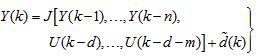 | (1) |
 is a nonlinear function of its arguments, and
 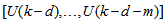 are the past input vector,
 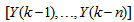 are the past output vector,
  is the current output,
  and
and  are the number of past inputs and outputs respectively that define the order of the system, and
  is time delay. The predictor form of (1) based on the information up to time
  can be expressed in the following compact form as [24, 25]:
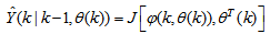 | (2) |

 is the regression (state) vector,
  is an unknown parameter vector which must be selected such that
  ,
,  is the error between (1) and (2) defined as
 | (3) |
 in
in  of (2) is henceforth omitted for notational convenience. Not that
  is the same order and dimension as
  .Now, let
  be a set of parameter vectors which contain a set of vectors such that:
 | (4) |
 is some subset of
  where the search for
  is carried out;
  is the dimension of
  ;
;  is the desired vector which minimizes the error in (3) and is contained in the set of vectors
 ;
;  are distinct values of
  ; and
; and  is the number of iterations required to determine the
  from the vectors in
  .Let a set of N input-output data pair obtained from prior system operation over NT period of time be defined:
 | (5) |
 | (6) |
 is formulated as a total square error (TSE) type cost function which can be stated as:
 | (7) |
 as an argument in
  is to account for the desired model
  dependency on
 . Thus, given as initial random value of
  ,
,  ,
,  and (5), the system identification problem reduces to the minimization of (6) to obtain
  . For notational convenience,
  shall henceforth be used instead of
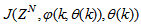 .
.4.2. Neural Network Identification Scheme
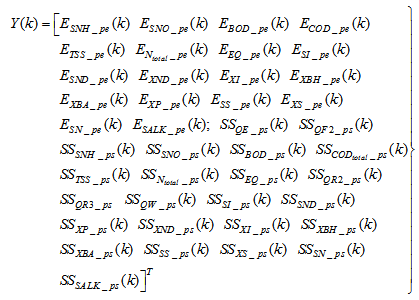
 | Figure 2. Architecture of the dynamic feedforward NN (DFNN) model |
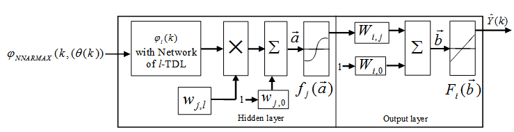
 | Figure 3. NN model identification based on the teacher-forcing method |
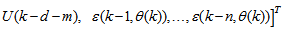
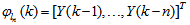
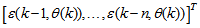
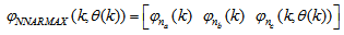
 as the desired model of network and having the DFNN architecture shown in Fig. 2. The proposed NN model identification scheme based on the teacher-forcing method is illustrated in Fig. 3. Note that the “Neural Network Model” shown in Fig. 3 is the DFNN shown in Fig. 2. The inputs to NN of Fig. 3 are
  ,
,  and
and 
 which are concatenated into
  as shown in Fig. 2. The output of the NN model of Fig. 3 in terms of the network parameters of Fig. 2 is given as:
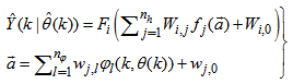 | (8) |
 and
and  are the number of hidden neurons and number of regressors respectively;
  is the number of outputs,
  and
and  are the hidden and output weights respectively;
  and
and  are the hidden and output biases;
  is a linear activation function for the output layer and
  is an hyperbolic tangent activation function for the hidden layer defined here as:
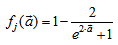 | (9) |
 is a collection of all network weights and biases in (8) in term of the matrices
  and
and . Equation (8) is here referred to as NN NARMAX (NNARMAX) model predictor for simplicity.Note that
  in (1) is unknown but is estimated here as a covariance noise matrix,
  Using
Using  , Equation (7) can be rewritten as:
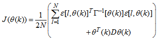 | (10) |
 is a penalty norm and also removes ill-conditioning, where
  is an identity matrix,
  and
and  are the weight decay values for the input-to-hidden and hidden-to-output layers respectively. Note that both
  and
and  are adjusted simultaneously during network training with
  and are used to update
  iteratively. The algorithm for estimating the covariance noise matrix and updating
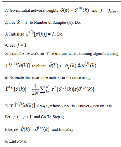
  is summarized in Table 2. Note that this algorithm is implemented at each sampling instant until
  has reduced significantly as in step 7).
|
|

4.3. Formulation of the Neural Network-Based ARLS Algorithm
- Unlike the BP which is a steepest descent algorithm, the ARLS and MLMA algorithms proposed here are based on the Gauss-Newton method with the typical updating rule [23, 25, 27, 28]:
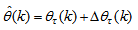 | (11) |
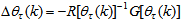 | (12) |
 denotes the value of
  at the current iterate
 is the search direction,
  and
and  are the Jacobian (or gradient matrix) and the Gauss-Newton Hessian matrices evaluated at
 .As mentioned earlier, due to the model
  dependency on the regression vector
  , the NNARMAX model predictor depends on a posteriori error estimate using the feedback as shown in Fig. 2. Suppose that the derivative of the network outputs with respect to
  evaluated at
  is given as
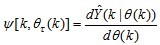 | (13) |
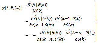 | (14) |
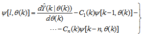 | (15) |
 , then (15) can be reduced to the following form
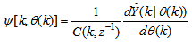 | (16) |
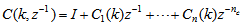
 which depends on the prediction error based on the predicted output. Equation (16) is the only component that actually impedes the implementation of the NN training algorithms depending on its computation.Due to the feedback signals, the NNARMAX model predictor may be unstable if the system to be identified is not stable since the roots of (16) may, in general, not lie within the unit circle. The approach proposed here to iteratively ensure that the predictor becomes stable is summarized in the algorithm of Table 3. Thus, this algorithm ensures that roots of
  lies within the unit circle before the weights are updated by the training algorithm proposed in the next sub-section.
4.3.1. The Adaptive Recursive Least Squares (ARLS) Algorithm
- The proposed ARLS algorithm is derived from (11) with the assumptions that: 1) new input-output data pair is added to
 progressively in a first-in first-out fashion into a sliding window, 2)
  is updated after a complete sweep through
 , and 3) all
  is repeated
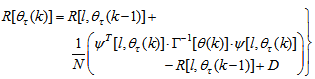
  times. Thus, Equation (10) can be expressed as [23], [30]:
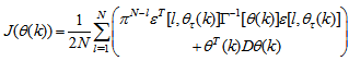 | (17) |
 is the exponential forgetting and resetting parameter for discarding old information as new data is acquired online and progressively added to the set
  .Assuming that
  minimized (17) at time
  ; then using (17), the updating rule for the proposed ARLS algorithm can be expressed from (11) as:
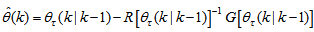 | (18) |
 and
and  given respectively as:
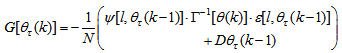
 | (19) |
 is computed according to (16).In order to avoid the inversion of
  , Equation (19) is first computed as a covariance matrix estimate,
  , as
, as 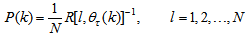 | (20) |
 By setting
 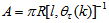 ,
,  and
and  , Equation (20) can also be expressed equivalently as
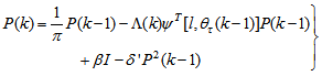 | (21) |
 is the adaptation factor given by
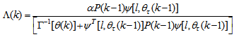 and I is an identity matrix of appropriate dimension,

 and
and  are four design parameters are selected such that the following conditions are satisfied [22], [23], 30]:
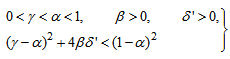 | (22) |
 in
in  adjusts the gain of the (21),
  is a small constant that is inversely related to the maximum eigenvalue of P(k),
  is the exponential forgetting factor which is selected such that
 and
and  is a small constant which is related to the minimum
  and maximum
  eigenvalues of (21) given respectively as [22], [23], [30], [31]:
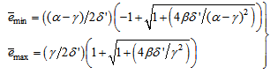 | (23) |


 and
and  in (22) is selected such that
 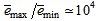 while the initial value of
 , that is
 , is selected such that
  [27].Thus, the ARLS algorithm updates based on the exponential forgetting and resetting method is given from (18) as
 | (24) |
 . Note that after
  has been obtained, the algorithm of Table 2 is implemented the conditions in Step 7) of the Table 2 algorithm is satisfied.
4.4. Proposed Validation Methods for the Trained Multivariable NNARMAX Model
- Network validations are performed to assess to what extend the trained network captures and represents the operation of the underlying system dynamics [25, 29].The first test involves the comparison of the predicted outputs with the true training data and the evaluation of their corresponding one-step ahead prediction errors using (3).The second validation test is the Akaike’s final prediction error (AFPE) estimate [25, 29] based on the weight decay parameter D in (10). A smaller value of the AFPE estimate indicates that the identified model approximately captures all the dynamics of the underlying system and can be presented with new data from the real process. Evaluating the
 portion of (3) using the trained network with
  and taking the expectation
  with respect to
  and
and  leads to the following AFPE estimate [23, 30, 31]:
 | (25) |
 and
and  is the trace of its arguments and it is computed as the sum of the diagonal elements of its arguments,
  and
and  is a positive quantity that improves the accuracy of the estimate and can be computed according to the following expression:
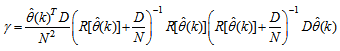 The third method is the K-step ahead predictions [10] where the outputs of the trained network are compared to the unscaled output training data. The K-step ahead predictor follows directly from (8) and for
 and
and , takes the following form:
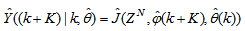 | (26) |


 The mean value of the K-step ahead prediction error (MVPE) between the predicted output and the actual training data set is computed as follows:
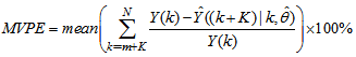 | (27) |
 corresponds to the unscaled output training data and
  the K-step ahead predictor output.
5. Integration and Formulation of the NN-Based AS-WWTP Problem
5.1. Selection of the Manipulated Inputs and Controlled Outputs of the AS-WWTP Process
- This section concentrates on the nonlinear model identification, predictions and control of the sludge height in the secondary settler and clarifier as well as the quality of the discharged effluent. The proposed scheme for the ANN-based nonlinear model identification and prediction, fuzzy rule-based decision system and intelligent adaptive control strategy for the for the sludge height in the secondary settler and clarifier as well the quality of the discharged effluent in the effluent tank of the AS-WWTP process is illustrated in Fig. 4.Case I: Nonlinear Model Identification and Prediction of the Sludge Height in the Secondary Settler and ClarifierThe objectives here is to maintain the quality and regulate the quantity of the disposed and recycled sludge by manipulating the feed flow rate (QF2 = 36892 m3.d-1) depending on the feed flow decision system, the RAS recycled flow rates (QR2 = 18446 m3.d-1 and QR3 = 18446 m3.d-1), and the WAS flow rate (QW = 385 m3.d-1) using TSS2, TSS3, TSS4, TSS5, TSS6, TSS7, TSS8, TSS9, and TSS10 as inputs with the following additional as inputs parameters: depending on the feed flow decision system using SI_s, SND_s, SNH_s, SNO_s, XND_s, XI_s, XBH_s, XBA_s, XP_s, SS_s, XS_s, SN_s, SALK_s, TSS_s as inputs.Case II: Nonlinear Model Identification and Prediction of the Effluent Quality in the Effluent TankThe objectives here is to maintain the quality and regulate the quantity of the discharged effluent by manipulating the effluent flow rate (QE = 18061 m3.d-1) and the feed flow rate (QF3 = 36892 m3.d-1) depending on the feed flow decision system using SI_e, SND_e, SNH_e, SNO_e, XND_e, XI_e, XBH_e, XBA_e, XP_e, SS_e, XS_e, SN_e, SALK_e, TSS_e as inputs.The European Union regulations and the COST 624 restrictions on effluent quality (EQ) stipulates that SNH_e = 4 gm-3, Ntotal_e = 17 gm-3, TSSE = 30 gm-3, BOD5_e = 2 gm-3, CODtotal,5_e = 48.2 gm-3, and EQ = 7550 kgd-1. These sixe parameters: SNH_e, Ntotal_e, TSSe, BOD5_e, CODtotal,5_e, and EQ have also been chosen as the constraint decision variables in this work.The ANN identification and prediction #1 block accepts its inputs from the effluent tank to generate the NN model and compute the predicted values of all the inputs. The constrained multi-objective optimization and decision block (Fig. 4) uses the predicted values to compute: SNH_e, Ntotal_e, TSSE, BOD5_e, CODtotal,5_e, and EQ. Based on the restricted effluent quality, genetic algorithm is used to perform the multi-objective optimization problem to determine the optimal values of the five constraint decision variables which forms the reference (set-point) values for the controlling and regulating the effluent quality and flow rate by the ANN identification, prediction and control #2 block (Fig. 4). This block also gives the final predicted values of the six parameters describing the effluent quality (SNH_e, Ntotal_e, TSSE, BOD5_e, CODtotal,5_e, and EQ) which would be used in future work to the compute the control signals to manipulate the following flow rates: Qinf, QE, QA1, QA2, QF1, QF2, QR1, QR2, QR3, and QW as well as QF12 and QR13.
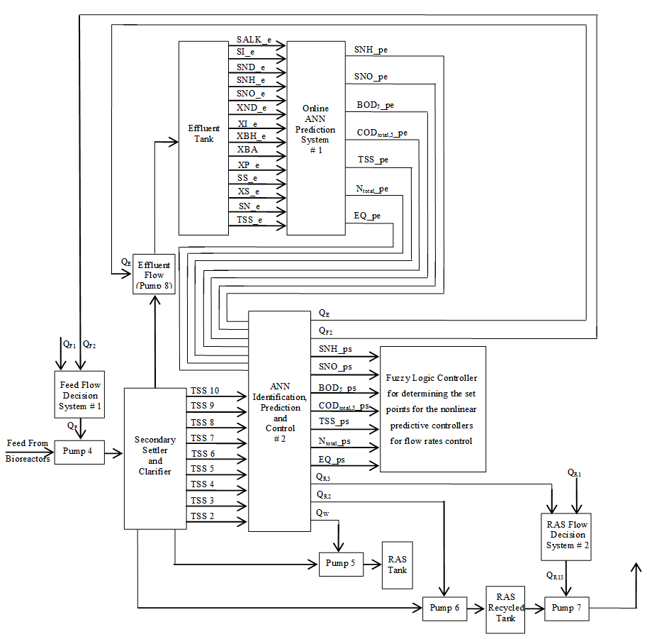 | Figure 4. The proposed scheme for the multivariable neural network-based NNARMAX model identification and prediction, fuzzy rule-based decision system and intelligent adaptive control strategy for the sludge height in the secondary settler and clarifier as well the quality of the discharged effluent in the effluent tank of the AS-WWTP process |
5.2. Formulation of the AS-WWTP Model Identification Problem
5.2.1. Statement of the AS-WWTP Neural Network Model Identification Problem
- The activated sludge wastewater treatment plant model defined by the benchmark simulation model no. 1 (BSM1) is described by eight coupled nonlinear differential equations given in Appendix A. The BSM1 model consist of thirteen states defined in Table 1 but they are redefined here for the effluent tank (with E and subscript e and pe for inputs and outputs respectively) as follows:
 and for the secondary settler (with SS and subscript s and ps for inputs and outputs respectively) as follows

 . Out of thirteen states, only four states are measurable namely:
  ,
,  (readily biodegradable substrate),
  (active heterotrophic biomass),
  (oxygen) and
 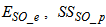 (nitrate and nitrite nitrogen). An additional important parameter
  and
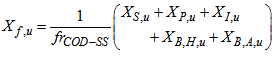
and  are used to assess the amount of soluble solids in the effluent tank and secondary settler/clarifier respectively.As highlighted above, the main objective here is on the efficient neural network model identification to obtain a multivariable NNARMAX model equivalent of the secondary settler/clarifier and the effluent tank of the activated sludge wastewater treatment plant (AS-WWTP) with a view in using the obtained model together with those from [22] to design a multivariable intelligent adaptive predictive control for the AS-WWTP process in our future work. Thus, from the discussions so far, the measured inputs that influence the behaviour of the AS-WWTP shown in Fig. 4 and Fig. 5 are:
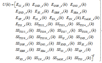 | (28) |
 | (29) |
 | Figure 5. The neural network model identification scheme for AS-WWTP based on NNARMAX model |
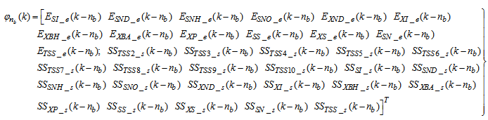
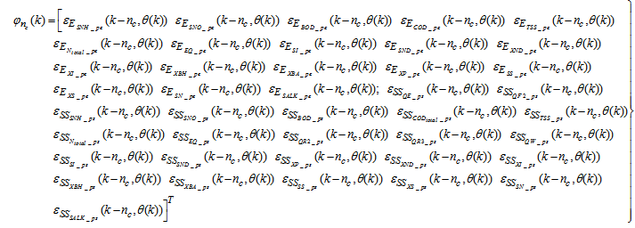
 for the NNARMAX models predictors discussed in Section 4 and defined here as Equation (30), (31), (32) and (33) below.The outputs of the neural network for the secondary settler with the clarifier and the effluent tank are the predicted values of the 13 states each together with the amount of total soluble solids (TSS), thus resulting in fourteen states; which together with the outputs of blocks #1 and #2 in Fig. 4 gives 41 outputs to be predicted at each sampling time instant as given in (34) below.
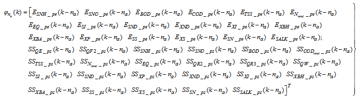 | (30) |
 | (31) |
 | (32) |
 | (33) |
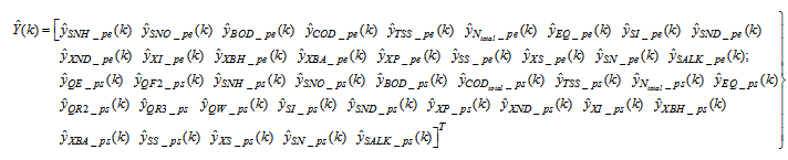 | (34) |
 affecting the AS-WWTP are incorporated into dry-weather data provided by the COST Action Group, additional sinusoidal disturbances with non-smooth nonlinearities are introduced for closed-loop performances evaluation based on an updated neural network model at each sampling time instants.
5.2.2. Experiment with the BSM1 for AS-WWTP Process Neural Network Training Data Acquisition
- For the efficient control of the activated sludge wastewater treatment plant (AS-WWTP) using neural network, a neural network (NN) model of the AS-WWTP process is needed which requires that the NN be trained with dynamic data obtained from the AS-WWTP process. In other to obtain dynamic data for the NN training, the validated and generally accepted COST Actions 624 benchmark simulation model no. 1 (BSM1) is implemented and simulated using MATLAB and Simulink as shown in Fig. 6. The BSM1 process model for the AS-WWTP process is given in Appendix A.A two-step simulation procedure defined in the simulation benchmark [2]–[4], [23] is used in this study. The first step is the steady state simulation using the constant influent flow (CONSTINFLUENT) for 150 days as shown and implemented in Fig. 6. Note that each simulation sample period indicated by the “Clock” of the AS-WWTP Simulink model in Fig. 6 corresponds to one day. In the second step, starting from the steady state solution obtained with the CONSTINFLUENT data and using the dry-weather influent weather data (DRYINFLUENT) as inputs, the AS-WWTP process is then simulated for 14 days using the same Simulink model of Fig. 6 but by replacing the CONSTINFLUENT influent data with the DRYINFLUENT influent data. This second simulation generates 1345 dynamic data in which is used for NN training while the 130 first day dry-weather data samples provided by the COST Actions 624 and 682 is used for the trained NN validation.
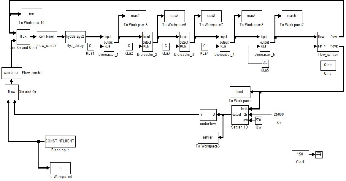 | Figure 6. Open-loop steady-state benchmark simulation model No.1 (BSM1) with constant influent |
5.2.3. The Incremental or Online Back-Propagation (INCBP) Algorithm
- In order to investigate the performance of the ARLS, the so-called incremental (or online) back-propagation (INCBP) algorithm is used for this purpose. The incremental or online back-propagation (INCBP) algorithm was originally proposed by [32] which has been modified in [23] is used in this paper. The incremental back-propagation (INCBP) algorithm is easily derived by setting the covariance matrix
 on the left hand side of (20) in Section 4.3.1 under the formulation of the ARLS algorithm; that is:
 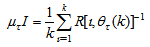 | (35) |
 is the step size and
  is an identity matrix of appropriate dimension. Next, the basic back-propagation given from [27] as:
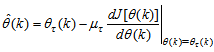 | (36) |
 and carry out the recursive computation of the gradient given by (36).
5.2.4. Scaling the Training Data and Rescaling the Trained Network that Models the AS-WWTP Process
- Due to the fact the input and outputs of a process may, in general, have different physical units and magnitudes; the scaling of all signals to the same variance is necessary to prevent signals of largest magnitudes from dominating the identified model. Moreover, scaling improves the numerical robustness of the training algorithm, leads to faster convergence and gives better models. The training data are scaled to unit variance using their mean values and standard deviations according to the following equations:
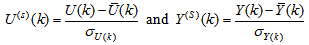 | (37) |

 and
and  ,
,  are the mean and standard deviation of the input and output training data pair; and
  and
and  are the scaled inputs and outputs respectively. Also, after the network training, the joint weights are rescaled according to the expression
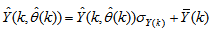 | (38) |
 and
and  shall be used.
5.2.5. Training the Neural Network that Models the Secondary Settler/Clarifier and Effluent Tank
- The NN input vector to the neural network (NN) is the NNARMAX model regression vector
 defined by (33). The input
 , that is the initial error estimates
  given by (32), is not known in advance and it is initialized to small positive random matrix of dimension
  by
by . The outputs of the NN are the predicted values of
  given by (34).For assessing the convergence performance, the network was trained for
  = 100 epochs (number of iterations) with the following selected parameters:
  ,
,  ,
,  ,
,  ,
,  ,
,  (NNARMAX),
  ,
,  ,
,  and
and . The details of these parameters are discussed in Section 3; where
  and
and  are the number of inputs and outputs of the system,
 and
and  are the orders of the regressors in terms of the past values,
  is the total number of regressors (that is, the total number of inputs to the network),
  and
and  are the number of hidden and output layers neurons, and
  and
and  are the hidden and output layers weight decay terms. The four design parameters for adaptive recursive least squares (ARLS) algorithm defined in (22) are selected to be: α=0.5, β=5e-3,
  =1e-5 and π=0.99 resulting to γ=0.0101. The initial values for ēmin and ēmax in (23) are equal to 0.0102 and 1.0106e+3 respectively and were evaluated using (23). Thus, the ratio of ēmin/ēmax from (23) is 9.9018e+4 which imply that the parameters are well selected. Also,
  is selected to initialize the INCBP algorithm given in (36).The 1345 dry-weather training data is first scaled using equation (37) and the network is trained for
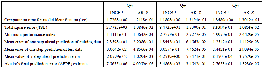
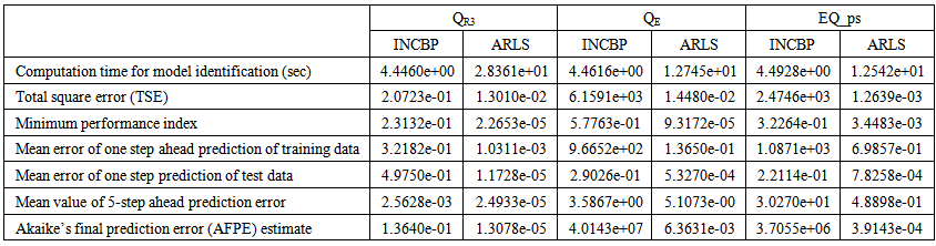
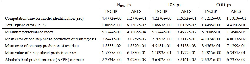
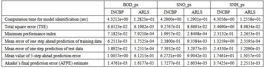
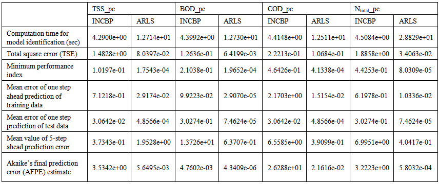
  epochs using the proposed adaptive recursive least squares (ARLS) and the incremental back-propagation (INCBP) algorithms proposed in Sections 4.3 and 5.2.3. After network training, the trained network is again rescaled respectively according to (38), so that the resulting network can work or be used with unscaled AS-WWTP data. Although, the convergence curves of the INCBP and the ARLS algorithms for 100 epochs each are not shown but the minimum performance indexes for both algorithms are given in the third rows of Tables 4 and 5 for the secondary settler/clarifier and effluent tank. As one can observe from these Tables, the ARLS has smaller performance index when compared to the INCBP which is an indication of good convergence property of the ARLS at the expense of higher computation time when compared the small computation time used by the INCBP for 100 epochs as evident in the first rows of Tables 4 and 5.The total square error (TSE) discussed in subsection 4.1, for the network trained with the INCBP and the ARLS algorithms are given in the second rows of Tables 4 and 5. Again, the ARLS algorithm also has smaller mean square errors and minimum performance indices when compared to the INCBP algorithm. The small values of the total square error (TSE) and the minimum performance indices indicate that ARLS performs better than the INCBP for the same number of iterations (epochs). These small errors suggest that the ARLS model approximates better the secondary settler/clarifier and effluent tank of the AS-WWTP process giving smaller errors than the INCBP model.
5.3. Validation of the Trained NNARMAX Model of the AS-WWTP Process
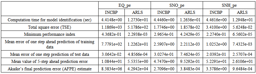
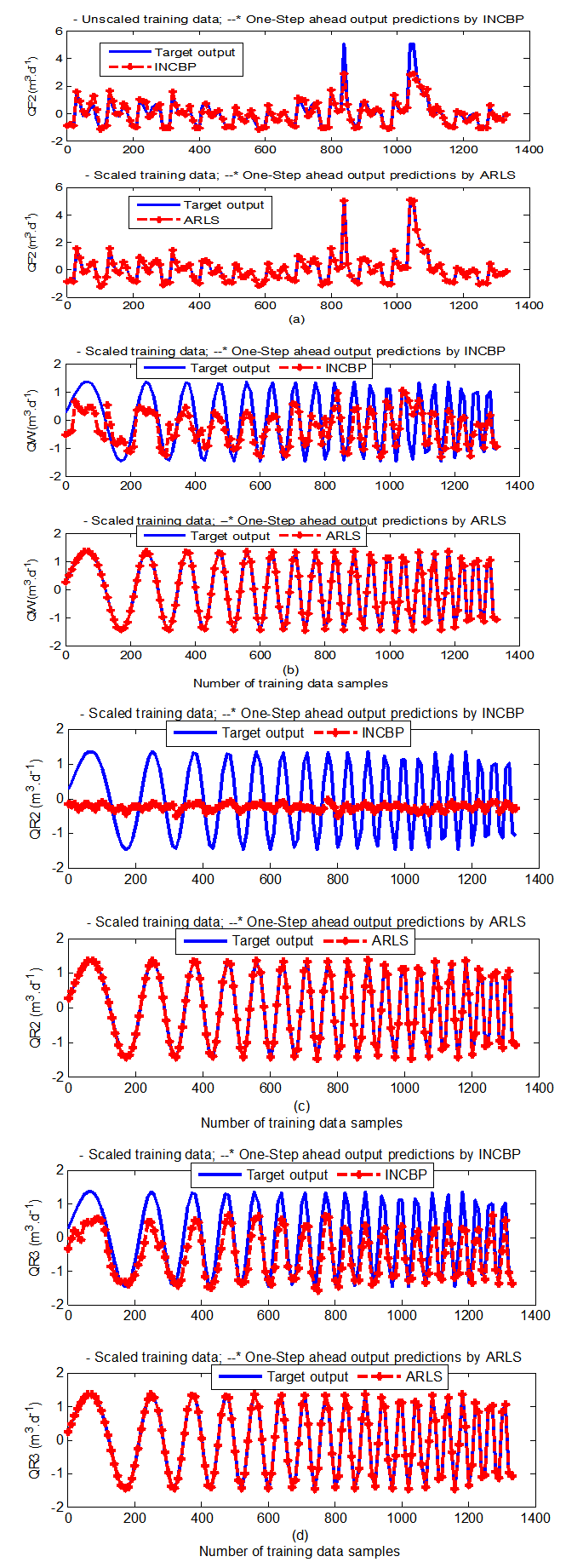
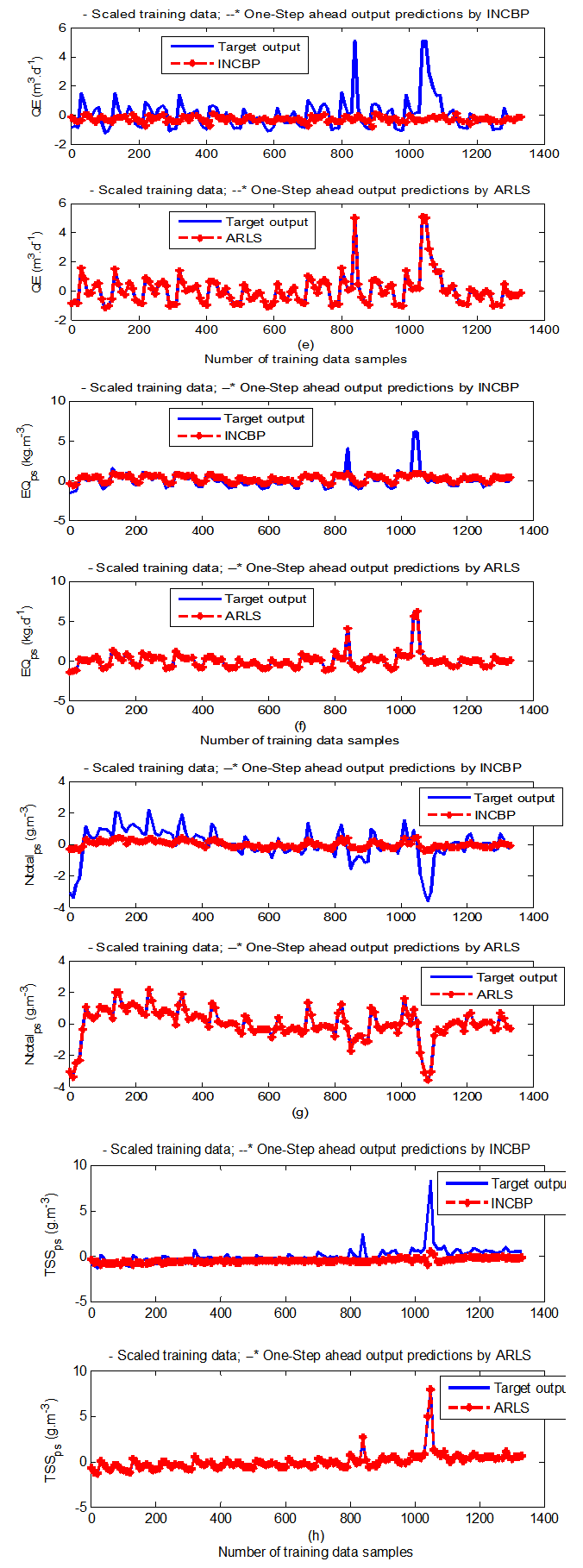
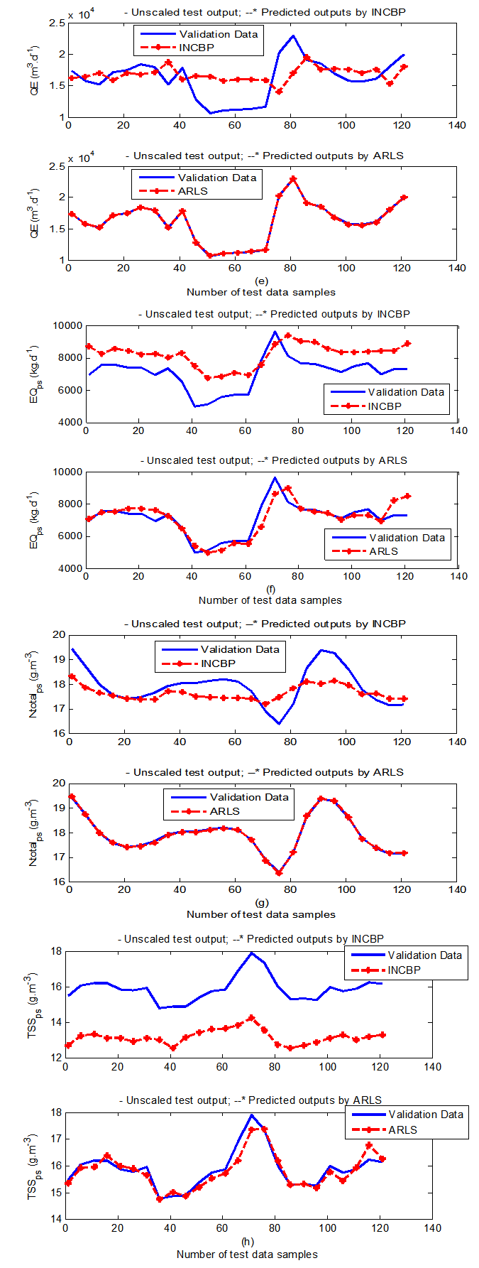
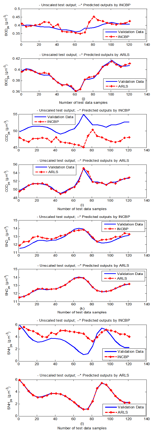
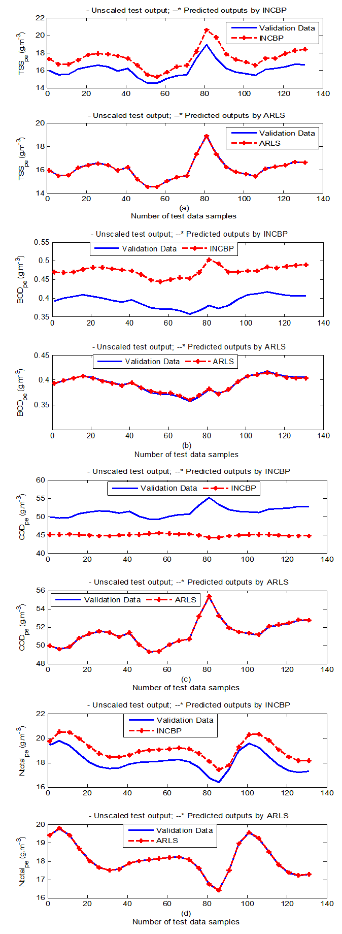
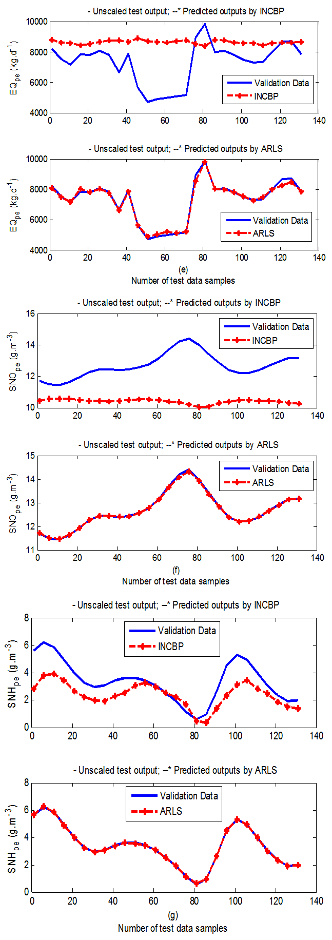
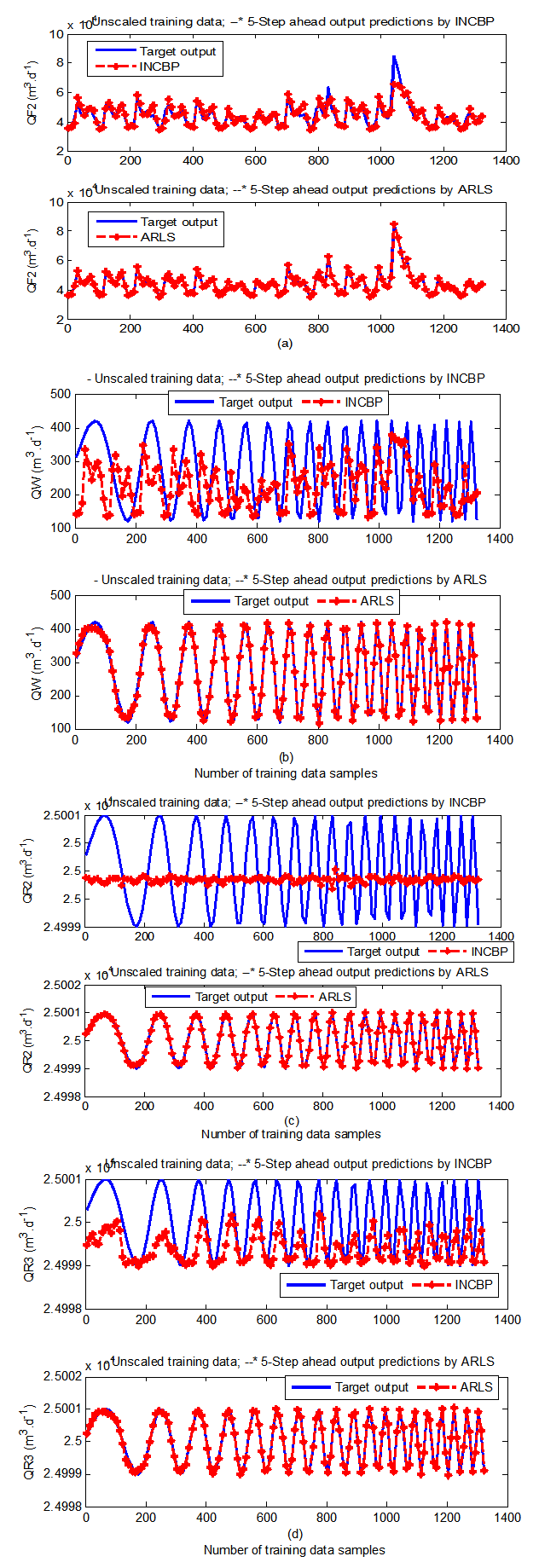
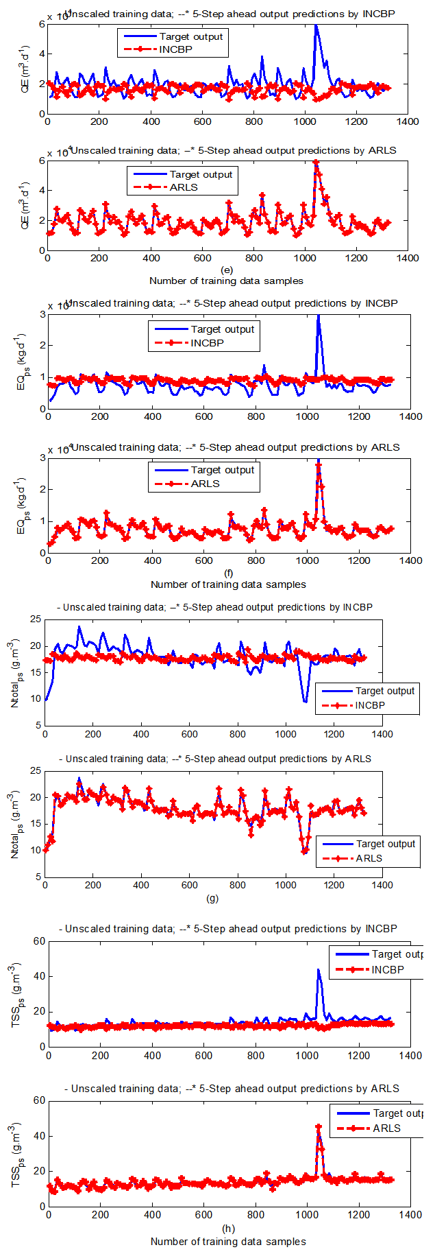
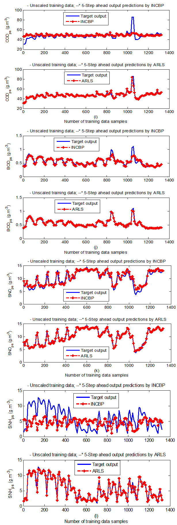
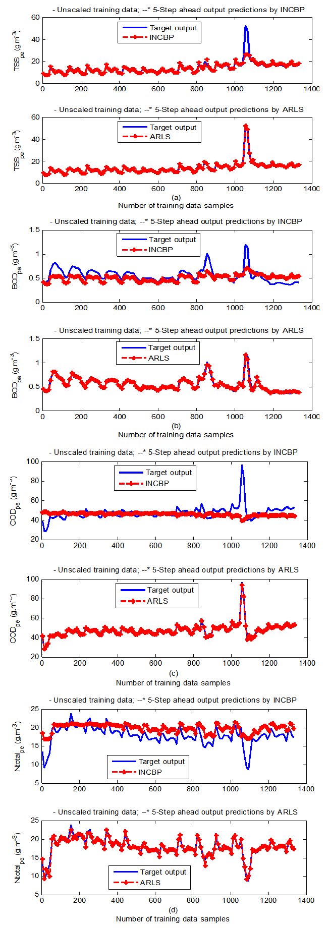
- According to the discussion on network validation in Section 4.4, a trained network can be used to model a process once it is validated and accepted, that is, the network demonstrates its ability to predict correctly both the data that were used for its training and other data that were not used during training. The network trained by the INCBP and the proposed ARLS algorithms has been validated with three different methods by the use of scaled and unscaled training data as well as with the 130 dry-weather data reserved for the validation of the trained network for the secondary settler/clarifier and effluent tank of the AS-WWTP process.The plots shown in (a) to (c) of Fig. 7, Fig. 8 and Fig. 9 corresponds to results obtained for the secondary settler and clarifier while those shown in (d) and (e) of Fig. 7, Fig. 8 and Fig. 9 are the results obtained for the effluent tank. The output parameters obtained in each of (a) to (e) were previously defined in Section 5.2.1 during the problem formulation but they are redefined here again as they appear in the next few figures (Fig. 7, Fig. 8 and Fig. 9) as follows:(a) is from the secondary settler and clarifier for QF2, QW, QR2 and QF3;(b) is from the secondary settler and clarifier for QE_ps, EQ_ps, Ntotal_ps and TSS_ps;(c) is from the secondary settler and clarifier for COD_ps, BOD_ps, SNO_ps and SNH_ps;(d) is from the effluent tank for TSS_pe, BOD_pe, COD_pe and Ntotal_pe;(e) is from the effluent tank for EQ_pe, SNO_pe and SNH_pe.The secondary settler and the clarifier depends on the following input parameters TSS2_s, TSS3_s, TSS4_s, TSS5_s, TSS6_s, TSS7_s, TSS8_s, TSS9_s, and TSS10_s together with the additional input parameter SI_s, SND_s, SNH_s, SNO_s, XND_s, XI_s, XBH_s, XBA_s, XP_s, SS_s, XS_s, SN_s, SALK_s, TSS_s as inputs to compute the outputs parameters given in (a), (b) and (c) above.The effluent tank depends on the following input parameters SI_e, SND_e, SNH_e, SNO_e, XND_e, XI_e, XBH_e, XBA_e, XP_e, SS_e, XS_e, SN_e, SALK_e, TSS_e as inputs to compute the outputs parameters given respectively in steps (d) and (e) above.In addition to the outputs given in (a) to (e) above, the following outputs parameters: SI_ps, SND_ps, SNH_ps, SNO_ps, XND_ps, XI_ps, XBH_ps, XBA_ps, XP_ps, SS_ps, XS_ps, SN_ps, SALK_ps, TSS_ps for the secondary settler and clarifier as well as SI_pe, SND_pe, SNH_pe, SNO_pe, XND_pe, XI_pe, XBH_pe, XBA_pe, XP_pe, SS_pe, XS_pe, SN_pe, SALK_pe, TSS_pe for the effluent tank are also predicted that are all used to compute the respective constraint parameters for the flow rates decision variables in order manipulating the pumps. The results for these additional outputs are not shown here for space economy rather only the results for the actual outputs are shown.
 | Table 4(a). Secondary settler and clarifier with the flow rates parameters predictions |
 | Table 4(b). Secondary settler and clarifier with the flow rates parameters predictions |
 | Table 4(c). Secondary settler and clarifier with the flow rates parameters predictions |
 | Table 4(d). Secondary settler and clarifier with the flow rates parameters predictions |
 | Table 5(a). Effluent tank and the effluent constrained parameters predictions |
 | Table 5(b). Effluent tank and the effluent constrained parameters predictions |
5.3.1. Validation by the One-Step Ahead Predictions Simulation
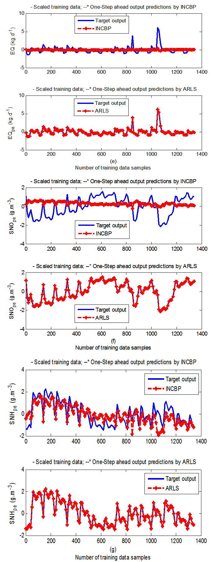
- In the one-step ahead prediction method, the errors obtained from one-step ahead output predictions of the trained network are assessed. In Fig. 7(a)–(e) the graphs for the one-step ahead predictions of the scaled training data (blue-) against the trained network output predictions (red --*) using the neural network models trained by INCBP and ARLS algorithms respectively are shown for 100 epochs.The mean value of the one-step ahead prediction errors are given in the fourth rows of Tables 4 and 5 respectively. It can be seen in the figures that the network predictions of the training data closely match the original training data. Although, the scaled training data prediction errors by both algorithms are small, the ARLS algorithm appears to have a much smaller error when compared to the INCBP algorithm as shown in the fourth rows of Tables 4 and 5. These small one-step ahead prediction errors are indications that the networks trained using the ARLS captures and approximate the nonlinear dynamics of the secondary settler/clarifier and effluent tank of the AS-WWTP process to a high degree of accuracy. This is further justified by the small mean values of the TSE obtained for the networks trained using the proposed ARLS algorithms for the process as shown in the second rows of Tables 4 and 5.Furthermore, the suitability of the INCBP and the proposed ARLS algorithms for neural network model identification for use in the real AS-WWTP industrial environment is investigated by validating the trained network with the 130 unscaled dynamic data obtained for dry-weather as provided by the COST Action Group. Graphs of the trained network predictions (red --*) of the validation (test) data with the actual validation data (blue -) using the INCBP and the proposed ARLS algorithms are shown in Fig. 8(a)–(e) for the secondary settler/clarifier and effluent tank of the AS-WWTP process based on the selected process parameters.The almost identical prediction of these data proves the effectiveness of the proposed approaches. The prediction accuracies of the unscaled test data by the networks trained using the INCBP and the proposed ARLS algorithm evaluated by the computed mean prediction errors shown in the fifth rows of Tables 4 and 5. Again, one can observe that although the validation data prediction errors obtained by both algorithms are small, the validation data predictions errors obtained with the model trained by the proposed ARLS algorithm appears much smaller when compared to those obtained by the model trained using the INCBP algorithm. These predictions of the unscaled validation data given in Fig. 8(a)–(e) as well as the mean value of the one step ahead validation (test) prediction errors in the fifth rows of Tables 4 and 5 verifies the neural network ability to model accurately the dynamics for the secondary settler/clarifier and effluent tank of the AS-WWTP process based on the dry-weather influent data using the proposed ARLS training algorithm.
 | Figure 7(a). One-step ahead prediction of scaled QF2, QW, QR2 and QF3 training data |
 | Figure 7(b). One-step ahead prediction of scaled QE_ps, EQ_ps, Ntotal_ps and TSS_ps training data |
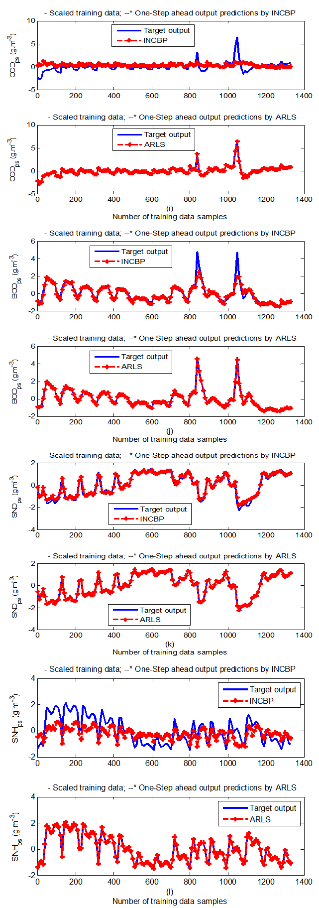 | Figure 7(c). One-step ahead prediction of scaled COD_ps, BOD_ps, SNO_ps and SNH_ps training data |
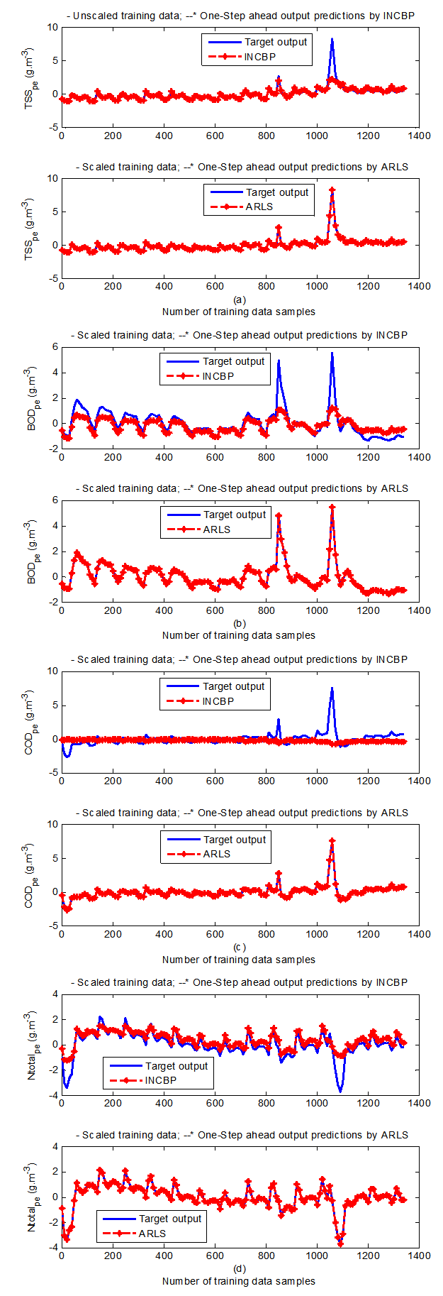 | Figure 7(d). One-step ahead prediction of scaled TSS_pe, BOD_pe, COD_pe and Ntotal_pe training data |
 | Figure 7(e). One-step ahead prediction of scaled EQ_pe, SNO_pe and SNH_pe training data |
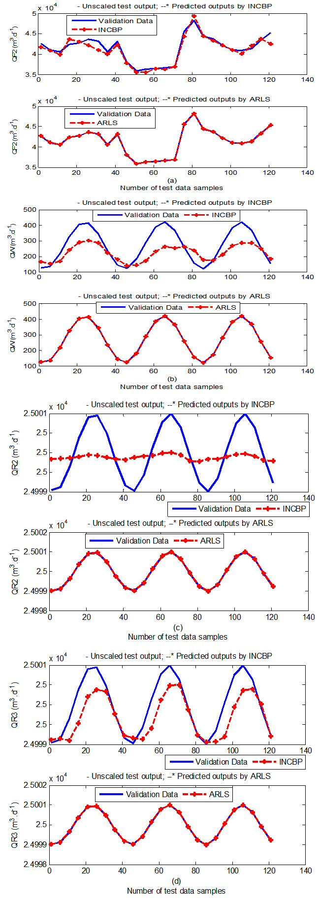 | Figure 8(a). One-step ahead prediction of unscaled QF2, QW, QR2 and QF3 validation data |
 | Figure 8(b). One-step ahead prediction of unscaled QE_ps, EQ_ps, Ntotal_ps and TSS_ps validation data |
 | Figure 8(c). One-step ahead prediction of unscaled COD_ps, BOD_ps, SNO_ps and SNH_ps validation data |
 | Figure 8(d). One-step ahead prediction of unscaled TSS_pe, BOD_pe, COD_pe and Ntotal_pe validation data |
 | Figure 8(e). One-step ahead prediction of unscaled EQ_pe, SNO_pe and SNH_pe validation data |
 | Figure 9(a). Five-step ahead prediction of unscaled QF2, QW, QR2 and QF3 training data |
 | Figure 9(b). Five-step ahead prediction of unscaled QE_ps, EQ_ps, Ntotal_ps and TSS_ps training data |
 | Figure 9(c). Five-step ahead prediction of unscaled COD_ps, BOD_ps, SNO_ps and SNH_ps training data |
 | Figure 9(d). Five-step ahead prediction of unscaled TSS_pe, BOD_pe, COD_pe and Ntotal_pe training data |
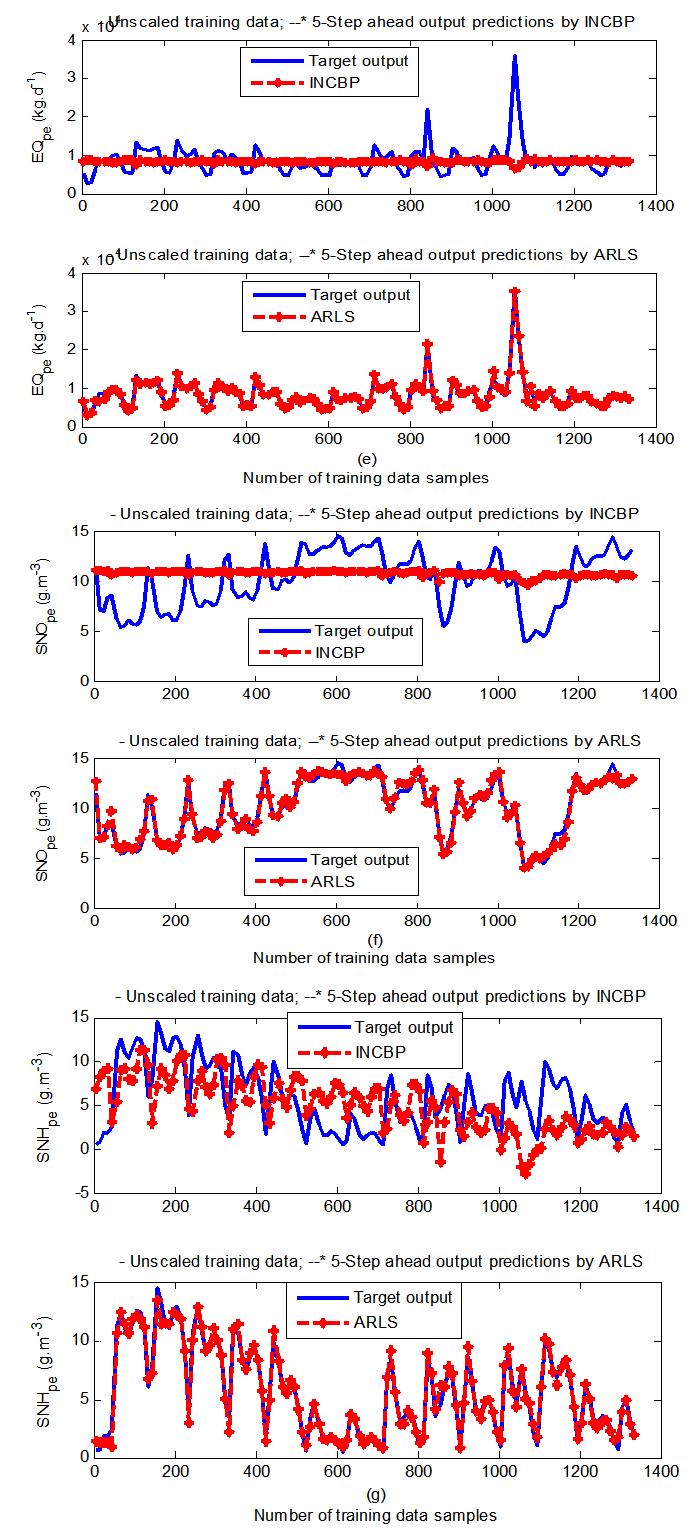 | Figure 9(e). Five-step ahead prediction of unscaled EQ_pe, SNO_pe and SNH_pe training data |
5.3.2. K–Step Ahead Prediction Simulations for the AS-WWTP Process
- The results of the K-step ahead output predictions (red --*) using the K-step ahead prediction validation method discussed in Section 4.4 for 5-step ahead output predictions (K = 5) compared with the unscaled training data (blue -) are shown in Fig. 9(a) to Fig. 9(e) for the networks trained using the INCBP and the proposed ARLS. Again, the value K = 5 is chosen since it is a typical value used in most model predictive control (MPC) applications. The comparison of the 5-step ahead output predictions performance by the network trained using the INCBP and the proposed ARLS algorithms indicate the superiority of the proposed ARLS over the so-called INCBP algorithm.The computation of the mean value of the K-step ahead prediction error (MVPE) using (27) is given in the sixth rows of Tables 4 and 5 by the network trained using INCBP and the proposed ARLS algorithms respectively. The small mean values of the 5-step ahead prediction error (MVPE) are indications that the trained network approximates the dynamics for the secondary settler/clarifier and effluent tank of the AS-WWTP process to a high degree of accuracy with the networks of both algorithms but with the network based on the ARLS algorithm giving much smaller distant prediction errors.
5.3.3. Akaike’s Final Prediction Error (AFPE) Estimates
- The implementation of the AFPE algorithm discussed in Section 4.4 and defined by (25) for the regularized criterion for the network trained using the INCBP and the proposed ARLS algorithms with multiple weight decay gives their respective AFPE estimates which are defined in the seventh rows of Tables 4 and 5 respectively. These relatively small values of the AFPE estimate indicate that the trained networks capture the underlying dynamics for the secondary settler/clarifier and effluent tank of the AS-WWTP and that the network is not over-trained [29]. This in turn implies that optimal network parameters have been selected including the weight decay parameters. Again, the results of the AFPE estimates computed for the networks trained using the proposed ARLS algorithm are much smaller when compared to those obtained using INCBP algorithm.
6. Conclusions
- This paper presents the formulation of an advanced online nonlinear adaptive recursive least squares (ARLS) model identification algorithm based on artificial neural networks for the nonlinear model identification of a AS-ASWWTP process. The mathematical model of the process obtained from COST Actions 632 and 624 has been simulated in open-loop to generate the training data while the First Day dry–weather data, also provided by the COST Actions group, is used as the validation (test) data. In order to investigate the performance of the proposed ARLS algorithm, the incremental backpropagation (INCBP), which is also an online algorithm, is implemented and its performance compared with proposed ARLS. The results from the application of these algorithms to the modeling of the secondary settler and the clarifier units of the AS-WWTP biological reactors as well as the validation results show that the neural network-based ARLS outperforms the INCBP algorithm with much smaller predictions error and good tracking abilities with high degree of accuracy and that the proposed ARLS model identification algorithm can be used for the AS-ASWWTP process in an industrial environment.The next aspect of the work is on the development of an adaptive fuzzy rule-based logic decision system which would produce the set points that can be used for the development of an intelligent multivariable nonlinear adaptive model-based predictive control algorithm for the efficient control of the complete AS-WWTP by manipulating the pumps based on the decision parameters discussed in this work.
Appendix
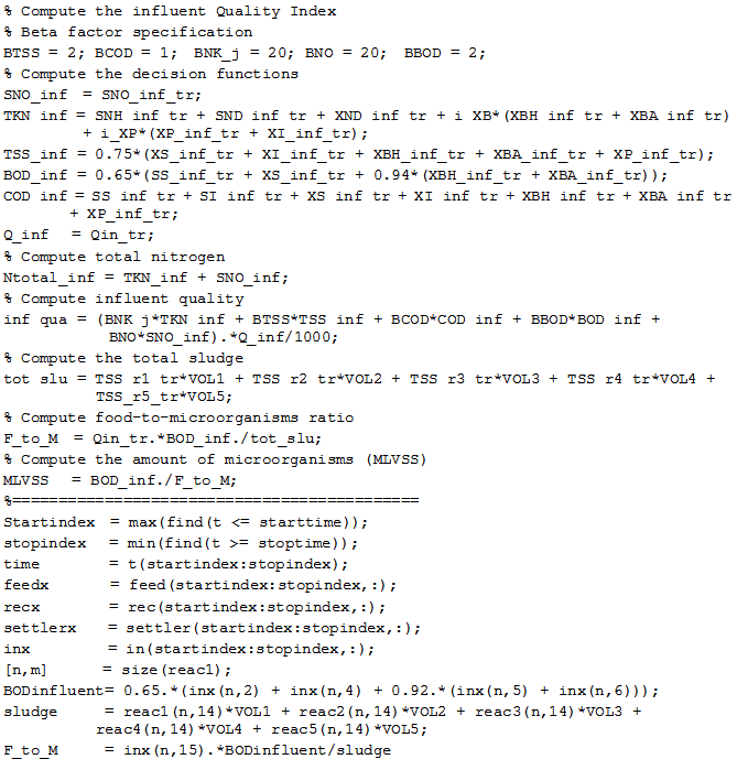
Appendix A: Computation of the Decision Parameters and Food-to-Microorganism Ratio
Appendix B: General Characteristics of the Secondary Settler and Clarifier
- Appendix B.1: Constructional Features
|
 . The height
  of each layer
  is
is , for a total height of
 . Therefore, the settler has total volume equal to
  .The solid flux due to gravity is
 | (B.1) |
 is the total sludge concentration and
  is a double-exponential settling velocity function defined as:
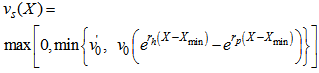 | (B.2) |
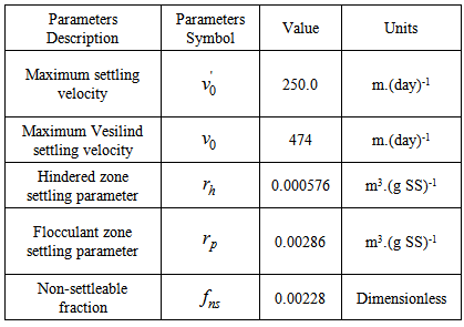
 . The parameter values for the non-exponential settling velocity function (B.2) are given in Table B.1. Thus, the mass balances for the sludge are expressed as:For the feed layer
  :
: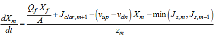 | (B.3) |
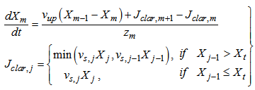
 to
to :
: | (B.4) |
 :
: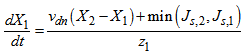 | (B.5) |
 to
to  :
: | (B.6) |
 :
: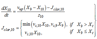 | (B.7) |
 .For the soluble components (including dissolved oxygen), each layer represents a completely mixed volume and the concentrations of soluble components are given accordingly as:For the feed layer
  :
: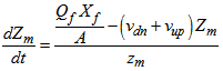 | (B.8) |
 to
to  :
: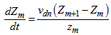 | (B.9) |
 to
to  :
: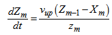 | (B.10) |
 | (B.11) |
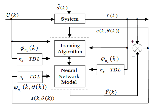
 , that is,
  .The sludge concentration from the concentrations in Unit 5 of Fig .1 can be computed from:
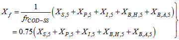 | (B.12) |
 . The same calculation is applied for
  in the settler underflow and
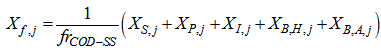
  at the plant exit.To calculate the distribution of particulate concentrations in the recycled and waste flows, their ratios with respect to the total solid concentration are assumed to remain constant across the settler:
 | (B.13) |
 ,
,  ,
,  ,
,  and
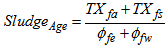
and  . The assumption made here means that the dynamics of the fractions of particulate concentrations in the inlet of the settler will be directly propagated to the settler underflow, without taking into account the normal retention time in the settler [1-4].Appendix B.2: Sludge AgeAppendix B.2.1: Sludge Age Based on Total Amount of BiomassIn the steady-state case, the sludge age calculation is based on the total amount of biomass present in the system that is in the reactor and settler:
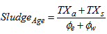 | (B.14) |
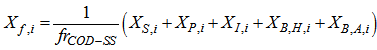
 is the total amount of biomass present in the reactor and it is expressed as:
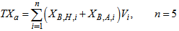 | (B.15) |
 is the total amount of biomass present in the effluent and it is expressed as:
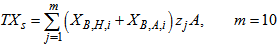 | (B.16) |
 is the loss rate of biomass in the effluent and it is expressed as:
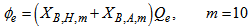 | (B.17) |
 is the loss rate of biomass in the waste flow and it is expressed as:
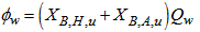 | (B.18) |
 | (B.19) |
 is the total amount of solids present in the reactor and can be expressed as:
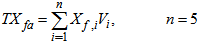 | (B.20) |
 | (B.21) |
 is the total amount of solids present in the settler and can be expressed as:
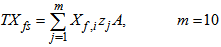 | (B.22) |
 | (B.23) |
 is the loss rate of solids in the effluent and can be expressed as:
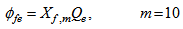 | (B.24) |
 | (B.25) |
 is the loss rate of solids in the waste flow and can be expressed as:
 | (B.26) |
Appendix C: Criteria for Evaluating and Assessing the Performances of the AS-WWTP Control
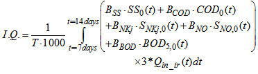
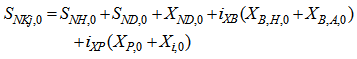
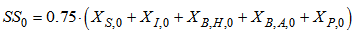
- Appendix C.1: Influent Quality (IQ)As a check on the IQ calculation, an influent quality index (IQ) can be calculated by applying the above equations to the influent file but the BOD coefficient must be changed from 0.25 to 0.65. It is defined as:
 | (C.1) |

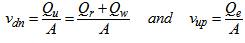
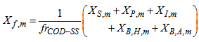
 Appendix C.2: Effluent Quality and ConstraintsAppendix C.2.1: Effluent Quality (EQ)The effluent quality (EQ), in kg pollution unit/d, is averaged over the period of observation
  (i.e. the second week or 7 last days for each weather file) based on a weighting of the effluent loads of compounds that have a major influence on the quality of the receiving water and that are usually included in regional legislation. It is defined as [2]–[4]:
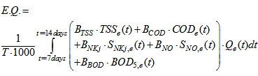 | (C.2) |


 where
where  are weighting factors for the different types of pollution to convert them into pollution units
  and were chosen to reflect these calculated fractions as follows:


 and
and The major operating cost in biological nutrient removal process as well as nitrogen removing ASPs is blower energy consumption. If the DO set-point is reduced by a control strategy, significant energy saving can be achieved. Operational issues are considered through three items: sludge production, pumping energy and aeration energy (integrations performed on the final 7 days of weather simulations (i.e. from day 22 to day 28 of weather file simulations,
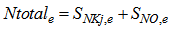
  ).Appendix C.2.2: Constraints on the Effluent QualityThe flow average values of the effluent concentrations over the three test periods (dry, rain and storm weather: 7 days for each) should be constrained for the five effluent components within the following limit: total nitrogen
  , total COD
  ammonia
 suspended solids
  and
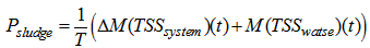
and  Appendix C.3: The Sludge production to be disposed (
 )This is the sludge production,
  is calculated from the total solid flow from wastage and solid accumulated in the system over the period of time considered (
 for each weather file). The amount of solids in the system at time t is given by:
  | (C.3) |
 is the amount of solids in the reactor given by:
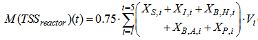 | (C.4) |
 is the amount of solids in the settler given by:
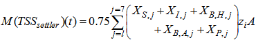 | (C.5) |
 the change in system sludge mass from the end of day 7 to the end of day 14 given by:
 and
and  the amount of waste sludge is given by:
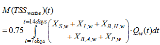 | (C.6) |
 | (C.7) |
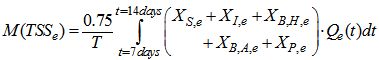
 )The total sludge production takes into account the sludge to be disposed and the sludge lost to the weir and is calculated as follows:
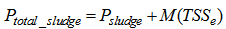 | (C.8) |
 Appendix C.5: The Pumping Energy (PE)The pumping energy in
  is calculated as follows:
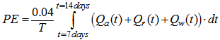 | (C.9) |
 is internal recycle flow rate at time
  is the return sludge recycle flow rate at time
  and
and  is the waste sludge flow rare at time
  Appendix C.6: The Aeration Energy (AE)The aeration energy (AE) in
  takes into account the plant peculiarities (type of diffuser, bubble size, depth of submersion, etc,) and is calculated from the
  in the three aerated tanks according to the following relation, valid for Degrémont DP230 porous disks at an immersion depth of 4m:
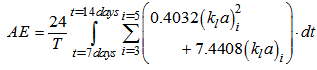 | (C.10) |
 is in
is in  and where i is the compartment number.The increase in capacity which could be obtained using the proposed control strategy should be evaluated. This factor is relative to investment costs if the plant would simply be extended to deal with increased load. This is expressed by the relative increase in the influent flow rate,
  which can be applied while maintaining the reference effluent quality index
  for the three weather conditions (
 days for each).
  is calculated from the above equation in open loop.
  with
with  for dry weather,
  for storm weather and
  for rain weather. Operation variables such as
  and
and  in compartments 3 and 4 remains unchanged.