1. Introduction

Wastewater flows are highly nonlinear and its measurements in terms of volume are accurately performed graphically using some obtained data. Wastewater variations can then be obtained by processing these data statistically. In situations where adequate measurements of the volume of wastewater are not available, it has been proposed in [1] that estimates and calculation should be performed; and for this purpose the wastewater is divided into typical three (3) parts: domestic wastewater, industrial and public institutions wastewater, and infiltration. Different analytical methods of a mixed origin are used for the characterization of wastewater and sludge as presented in [1], and many of them have been specially developed for treatment plants and treatment processes. Wastewater normally contains thousands of different organics and a measurement of each individual organic matter would be impossible rather a different collective analyses are used which comprise a greater or minor part of the organics. Activated sludge wastewater treatment processes (ASWWTP) are difficult to control because of their complexity; nonlinear behaviour; large uncertainty in uncontrolled inputs and in the model parameters and structure; multiple time scales of the dynamics and multivariable input-output structure. The first control opportunity in ASWWTP is regulating the influent flow-rate which implies that control issues in wastewater treatment facilities pertain primarily to aeration control for energy usage and satisfying process demands.

The most straightforward controller design techniques are those that are based on a linear mathematical model of the controlled process [2]. However, the characteristics of the ASWWTP processes are highly nonlinear and time-varying in nature. In these cases the linear controller design techniques result to inefficient control algorithms [3] and methods based on nonlinear models of the processes are preferred [4], [5]. In either of the linear or nonlinear cases, the use of a model of the process does not fully reflect the actual process operation over long periods of time. Therefore, the algorithms obtained by controller design techniques which are based on a mathematical model of the controlled process [2] are not very efficient because these methods cannot guarantee stable control outside the range of the model validity [3], [6]. For these reasons adaptive algorithms which could be based on a continuous model updating process and redesign of the control strategy before a new control action is applied to the real plant would result to a better plant performance.

Even if this approach is adopted, the application of traditional modeling methods used in several variations of the controller designs, such as those reported in [7]–[9], cannot model accurately the strong interactions among the process variables as well as the short and tight operating constraints. The best approach would be the use of highly complicated validated models of groups of nonlinear differential and partial differential equations, and the invention of new control design methods based on these models. However the computational burden for modeling dynamic systems with relatively short sampling interval becomes enormous to be handled even by the new multi-core, clustering and field programmable gate array (FPGA) technologies. In order to exploit these technologies, instead of using groups of differential equations, one could consider developing other accurate nonlinear models, the computational burden of which would be of course higher than the linear models but less than that of the groups of differential equations.

A recent approach to modeling nonlinear dynamical systems is the use of neural networks (NN). The application of neural networks (NN) for model identification and adaptive control of dynamic systems has been studied extensively [6], [10]–[19]. As demonstrated in [13], [14], [16], and [17], neural networks can approximate any nonlinear function to an arbitrary high degree of accuracy. The adjustment of the NN parameters results in different shaped nonlinearities achieved through a gradient descent approach on an error function that measures the difference between the output of the NN and the output of the true system for given input data or input-output data pairs (training data).

In the absence of operating data from the transient and steady state operation of the system to be controlled, data for training and testing the NN model can be obtained from the system by simulating the validated model of the groups of differential equations which are usually derived from the first principles on which the operation of the physical process is based. Such approaches are reported in [6], [10], 18], [21]. The use of the nonlinear NN models can replace the first principles model equally well and it can reduce the computational burden as argued in [21], [22]. This is because a nonlinear discrete NN model of high accuracy is available immediately after or at each instant of the network training process.

The aim of the paper is on the efficient modeling of a nonlinear neural network autoregressive moving average with exogenous input (NNARMAX) model that will capture the nonlinear dynamics of an activated sludge wastewater treatment plant (AS-WWTP) for the purpose of developing an efficient nonlinear adaptive controller for the efficient control of the AS-WWTP process. Due to the multivariable nature of the AS-WWTP, the present paper (Part 1) considers the modeling of the five biological reactors including the influent tank while the second paper (Part 2) will be devoted to the modeling of the secondary settler and clarifier as well as the effluent tank.

2. The AS-WWTP Process Description

2.1. Overview of the AS-WWTP Process

The activated sludge process was developed in England in 1914 by Arden and Lockett (Arden, et al.) and was so named because in involved the production of an activated mass of microorganisms capable of aerobically stabilizing a waste. The activated sludge process has been utilized for treatment of both domestic and industrial wastewaters for over half a century. This process originated from the observation made a long time ago that whenever wastewater, either domestic or industrial, is aerated for a period of time, the content of organic matter is reduced, and at the same time a flocculent sludge is formed. Microscopic examination of this sludge reveals that it is formed by a heterogenous population of microorganisms, which changes continually in nature in response to variation in the composition of the wastewater and environmental conditions. Microorganisms present are unicellular bacteria, fungi, algae, protozoa, and rotifiers.

Organic wastewater is introduced into a reactor where an aerobic bacterial culture is maintained in suspension. The reactor contents are referred to as the mixed liquor. In the reactor, the bacterial culture converts the organic content of the wastewater into cell tissue. The aerobic environment in the reactor is achieved by the use of diffused or mechanical aeration, which also serve to maintain the liquor in a completely mixed regime. After a specified period of time, the mixture of new cells and old cells is passed into a settling tank where the cells are separated from the treated wastewater. A portion of the settled cells is recycled to maintain the desired concentration of organisms in the reactor, and a portion is wasted.

Traditionally, activated sludge process (ASP) involve an anaerobic (anoxic) followed by an aerobic zone and a settler from which the major part of the biomass is recycled to the anoxic basin and this prevents washout of the process by decoupling the sludge retention time (SRT) from the hydraulic retention time (HRT). Activated sludge wastewater treatment plants (ASWWTP) are built remove organic mater from wastewater where a bacterial biomass suspension (the activated sludge) is responsible for the removal of pollutants. Depending on the design and specific application, ASTP can achieve biological nitrogen removal, biological phosphorus removal and removal of organic carbon substances as well as the amount of dissolved oxygen [23]. Generally, an ASWWTP can generally be regarded as a complex system [24]–[26] due to its highly nonlinear dynamics, large uncertainty, multiple time scales in the internal processes as well as its multivariable structure. A widely accepted biodegradation model is the activated sludge model no. 1 (ASM1) which incorporates the basic biotransformation processes of an activated sludge wastewater treatment plant [1], [27]–[30].

The objective of the activated sludge process is to achieve a sufficiently low concentration of biodegradable matter in the effluent together with minimal sludge production at minimal cost. Although the operation of the ASP for wastewater treatment plants is challenging for both economical and technical reasons but the basic principle in activated sludge plants is that a mass of activated sludge is kept moving in water by stirring or aeration. Apart from the living biomass, the suspended solids contain inorganic as well as organic particles. While some of the organic particles can be degraded through hydrolysis, the others are non-degradable (inert). The amount of suspended solids in the treatment plant is regulated through recycle of the suspended solids and by removing the so-called excess sludge. The purpose of recycle is to increase the sludge concentration in the aeration tank which results in an increase sludge age as the hydraulic retention time and the sludge age are separated. In this way it is possible to accumulate a biomass consisting of both rapid- and slow-growing micro-organisms which is very important for the settling and flocculation behaviour of the sludge.

The activated sludge process is a treatment technique in which wastewater and reused biological sludge full of living microorganisms are mixed and aerated. The biological solids are then separated from the treated wastewater in a clarifier and are returned to the aeration process or wasted. The microorganisms are mixed thoroughly with the incoming organic material, and they grow and reproduce by using the organic material as food. As they grow and are mixed with air, the individual organisms clings together (flocculate). Once flocculated, they more readily settle in the secondary clarifiers. The wastewater being treated flows continuously into an aeration tank where air is injected to mix the wastewater with the returned activated sludge and to supply the oxygen needed by the microbes to live and feed on the organics. Aeration can be supplied by injection through air diffusers in the bottom of tank or by mechanical aerators located at the surface.

The mixture of activated sludge and wastewater in the aeration tank, mixed liquor, flows to a secondary clarifier where the activated sludge is allowed to settle. The activated sludge is constantly growing, and more is produced than can be returned for use in the aeration basin. Some of this sludge must be wasted to a sludge handling system for treatment and disposal (solids) or reuse (bio-solids). The volume of sludge returned to the aeration basins is normally 40 to 60% of the wastewater flow while the rest is wasted (solids) or reuse (bio-solids).

A number of factors affect the performance of an activated sludge system. These include the following: (i) temperature, (ii) return rates, (iii) amount of oxygen available, (iv) amount of organic matter available, (v) pH, (vi) waste rates, (vii) aeration time and (viii) wastewater toxicity. To obtain the desired level of performance in an activated sludge system, a proper balance must be maintained between the amount of food (organic matter), organisms (activated sludge), and dissolved oxygen (DO). The majority of problems with the activated sludge process result from an imbalance between these three items. The actual operation of an activated-sludge system is regulated by three factors: 1) the quantity of air supplied to the aeration tank; 2) the rate of activated-sludge recirculation; and 3) the amount of excess sludge withdrawn form the system. Sludge wasting is an important operational practice because it allows the establishment of the desired concentration of mixed liquor soluble solids (MLSS), food to microorganisms ratio (F : M ratio), and sludge age. It should be noted that air requirements in an activated sludge basin are governed by: 1) BOD loading and the desired removal effluent, 2) volatile suspended solids concentration in the aerator, and 3) suspended solids concentration of the primary effluent.

2.2. Description of the AS-WWTP Process

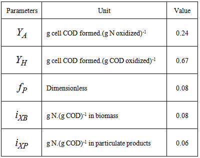
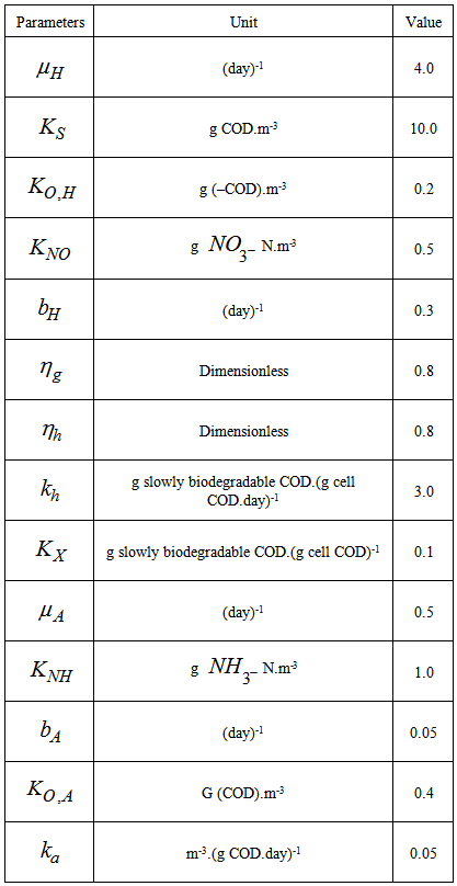
Activated sludge wastewater treatment plants (WWTPs) are large complex nonlinear multivariable systems, subject to large disturbances, where different physical and biological phenomena take place. Many control strategies have been proposed for wastewater treatment plants but their evaluation and comparison are difficult. This is partly due to the variability of the influent, the complexity of the physical and biochemical phenomena, and the large range of time constants (from a few minutes to several days) inherent in the activated sludge process. Additional complication in the evaluation is the lack of standard evaluation criteria.

With the tight effluent requirements defined by the European Union and to increase the acceptability of the results from wastewater treatment analysis, the generally accepted COST Actions 624 and 682 benchmark simulation model no. 1 (BSM1) model [1] is considered. The BSM1 model uses eight basic different processes to describe the biological behaviour of the AS-WWTP processes. The combinations of the eight basic processes results in thirteen different observed conversion rates as described in Appendix A. These components are classified into soluble components (S) and particulate components (X). The nomenclatures and parameter definitions used for describing the AS-WWTP in this work are given in Table 1. Moreover, four fundamental processes are considered: the growth and decay of biomass (heterotrophic and autotrophic), ammonification of organic nitrogen and the hydrolysis of particulate organics. The complete BSM1 used to describe the AS-WWTP considered here is given in Appendix A while the general characteristics of the biological reactors are given in Appendix B. Additional information on the complete mathematical modeling of the AS-WWTP considered here can be found in [27].

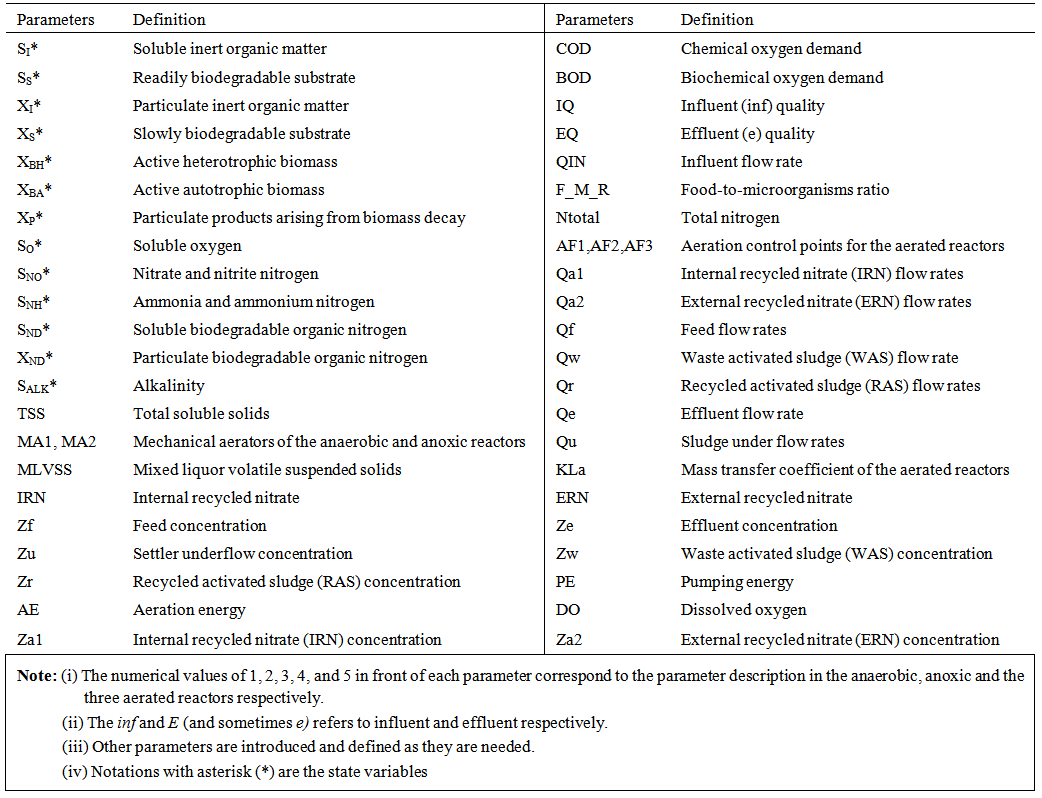Table 1. The AS-WWTP Nomenclatures and Parameter Definitions

The schematic of a BNR-ASWWTP design with basic control strategies is shown in Fig.1 using the Johannesburg configuration [24], [25] which consists of anaerobic, anoxic and aerobic zones and a secondary settler in a back-to-back scheme with multiple recycle streams [27]. To ensure that plug flow conditions prevail in the bioreactors, the basins are usually partitioned such that back-mixing is minimized. The constructional features and nomenclature of the process is detailed in Appendix C of [27]. Nevertheless, the biological processes within the different zones of the reactors are briefly presented in the following.

Figure 1. The schematic of the AS-WWTP process

In the anaerobic zone, fermentable organic from the influent wastewater are mixed with the return-activated sludge (RAS) and converted to volatile fatty acids (VFA) by heterotrophic organisms. The latter is consumed by phosphorus-accumulating organisms (PAO) and stored internally as poly-β hydroxy alkanoates (PHA). Concurrently, poly phosphate and hence energy for VFA accumulation are internally released. Denitrification in this zone results in a net reduction of alkalinity and hence there is an increase in pH due to acids production. If the amount of VFA is insufficient, additional acids from external source may be added to maintain a maximum PHA uptake by the biological phosphate organisms. It is also common to install an activated primary sedimentation tank to allow production of VFA by fermentation of readily substrate in the incoming sewage.

In the anoxic zone, nitrate (S_NO) which is recycled from the aerobic zone is converted to dinitrogen by facultative heterotrophic organisms. Denitrification in this zone results in the release of alkalinity and hence there is an increase in pH value. There is also evidence of a pronounced removal of phosphorus in this zone.

In the partially-treated wastewater arriving the aerobic zone, virtually al the readily biodegradable organic (referred to as biodegradable COD) in the partially-treated wastewater has been consumed by heterotrophic organisms in the aerobic and anoxic zones. Thus in this aerobic zone, two major processes occur. In the presence of dissolved oxygen (S_O), the released phosphate is taken up by PAO growing on the stored PHA. The phosphorus is stored internally as poly phosphate. This results in a net reduction in phosphate in the wastewater. The second process occurring in this zone is nitrification of ammonia to nitrate in the wastewater by the autotrophic organisms. In order to minimize the amount of DO going into the anoxic zone, the last compartment is typically aerated. Part of the sludge, which contains phosphorus to be removed, is wasted while the remainder is returned to the anaerobic zone after thickening in the settler and additional denitrification in the RAS tank.

The activated sludge wastewater treatment plant considered here is strictly based on the benchmark simulation model no. 1 (BSM1) proposed by the European Working Groups of COST Action 624 and 682 in conjunction with the International Water Association (IWA) Task Group on Benchmarking of Control Strategies for wastewater treatment plants (WWTPs) [28], [29]. This implementation of the benchmark simulation model no. 1 (BSM1) follows the methodology specified in [27]–[29] especially from the viewpoint of control performances. The complete description of the conventional activated sludge wastewater treatment plant (AS-WWTP) based on the benchmark simulation model no. 1 (BSM1) is given in Appendix C of [27] together with the mathematical model of the benchmark simulation model no. 1 (BSM1) and the MATLAB/Simulink programs that implements the mathematical model of the BSM1.

3. The Neural Network Identification Scheme and Validation Algorithms

3.1. Formulation of the Neural Network Model Identification Problem

The method of representing dynamical systems by vector difference or differential equations is well established in systems [30], [31] and control [12], [13], [32], [33] theories. Assuming that a p-input q-output discrete-time nonlinear multivariable system at time with disturbance can be represented by the following Nonlinear AutoRegressive Moving Average with eXogenous inputs (NARMAX) model [30], [31]:

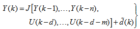(1)

where is a nonlinear function of its arguments, and 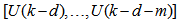are the past input vector, 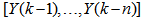are the past output vector, is the current output, and are the number of past inputs and outputs respectively that define the order of the system, and is time delay. The predictor form of (1) based on the information up to time can be expressed in the following compact form as [30], [31]:

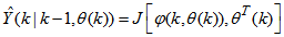(2)

where is the regression (state) vector, is an unknown parameter vector which must be selected such that , is the error between (1) and (2) defined as

(3)

where in of (2) is henceforth omitted for notational convenience. Not that is the same order and dimension as.

Now, let be a set of parameter vectors which contain a set of vectors such that:

(4)

where is some subset of where the search for is carried out; is the dimension of ; is the desired vector which minimizes the error in (3) and is contained in the set of vectors ; are distinct values of ; and is the number of iterations required to determine the from the vectors in .

Let a set of input-output data pair obtained from prior system operation over NT period of time be defined:

(5)

where is the sampling time of the system outputs. Then, the minimization of (3) can be stated as follows:

(6)

where is formulated as a total square error (TSE) type cost function which can be stated as:

(7)

The inclusion of as an argument in is to account for the desired model dependency on. Thus, given as initial random value of , m, n and (5), the system identification problem reduces to the minimization of (6) to obtain. For notational convenience, shall henceforth be used instead of.

3.2. Neural Network Identification Scheme

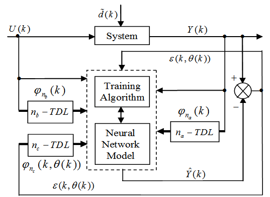
The minimization of (6) is approached here by considering as the desired model of network and having the DFNN architecture shown in Fig. 2. The proposed NN model identification scheme based on the teacher-forcing method is illustrated in Fig. 3. Note that the “Neural Network Model” shown in Fig. 3 is the DFNN shown in Fig. 2. The inputs to NN of Fig. 3 are , and which are concatenated into as shown in Fig. 2. The output of the NN model of Fig. 3 in terms of the network parameters of Fig. 2 is given as:

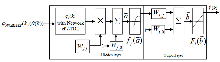Figrue 2. Architecture of the dynamic feedforward NN (DFNN) model

Figure 3. NN model identification based on the teacher-forcing method

(8)

where and are the number of hidden neurons and number of regressors respectively; is the number of outputs, and are the hidden and output weights respectively; and are the hidden and output biases; is a linear activation function for the output layer and is an hyperbolic tangent activation function for the hidden layer defined here as:

(9)

Bias is a weight acting on the input and clamped to 1. Here, is a collection of all network weights and biases in (8) in term of the matrices and . Equation (8) is here referred to as NN NARMAX (NNARMAX) model predictor for simplicity.

Note that in (1) is unknown but is estimated here as a covariance noise matrix, Using, Equation (7) can be rewritten as:

(10)

where the second term in (10) is the regularization (weight decay) term [31] which has been introduced to reduce modeling errors, improve the robustness and performance of the two proposed training algorithms. is a penalty norm and also removes ill-conditioning, where is an identity matrix, and are the weight decay values for the input-to-hidden and hidden-to-output layers respectively. Note that both and are adjusted simultaneously during network training with and are used to update iteratively. The algorithm for estimating the covariance noise matrix and updating is summarized in Table 2. Note that this algorithm is implemented at each sampling instant until has reduced significantly as in step 7).

3.3. Formulation of the Neural Network-Based ARLS Algorithm

Unlike the BP which is a steepest descent algorithm, the ARLS and MLMA algorithms proposed here are based on the Gauss-Newton method with the typical updating rule [30]–[34]:

(11)

where

(12)

denotes the value of at the current iterate is the search direction, and are the Jacobian (or gradient matrix) and the Gauss-Newton Hessian matrices evaluated at .

As mentioned earlier, due to the model dependency on the regression vector, the NNARMAX model predictor depends on a posteriori error estimate using the feedback as shown in Fig. 2. Suppose that the derivative of the network outputs with respect to evaluated at is given as

(13)

The derivative of (13) is carried out in a BP fashion for the input-to-hidden layer and for the hidden-to-output layer respectively for the two-layer DFNN of Fig. 2. Thus, the derivative of the NNARMAX model predictor can be expressed as

(14)

Thus, Equation (14) can be expressed equivalently as

(15)

By letting , then (15) can be reduced to the following form

(16)

As it can be seen from (16), the gradient is calculated by filtering the partial derivatives with the time-varying filter which depends on the prediction error based on the predicted output. Equation (16) is the only component that actually impedes the implementation of the NN training algorithms depending on its computation.

Due to the feedback signals, the NNARMAX model predictor may be unstable if the system to be identified is not stable since the roots of (16) may, in general, not lie within the unit circle. The approach proposed here to iteratively ensure that the predictor becomes stable is summarized in the algorithm of Table 3. Thus, this algorithm ensures that roots of lies within the unit circle before the weights are updated by the training algorithm proposed in the next sub-section.

3.3.1. The Adaptive Recursive Least Squares (ARLS) Algorithm

The proposed ARLS algorithm is derived from (11) with the assumptions that: 1) new input-output data pair is added to progressively in a first-in first-out fashion into a sliding window, 2) is updated after a complete sweep through , and 3) all is repeated times. Thus, Equation (10) can be expressed as [27], [35]:

(17)

is the exponential forgetting and resetting parameter for discarding old information as new data is acquired online and progressively added to the set .

Assuming that minimized (17) at time; then using (17), the updating rule for the proposed ARLS algorithm can be expressed from (11) as:

(18)

where and given respectively as:

(19)

where is computed according to (16).

In order to avoid the inversion of, Equation (19) is first computed as a covariance matrix estimate, , as

(20)

Then, by using the following matrix inversion lemma:

By setting , and , Equation (20) can also be expressed equivalently as

(21)

where is the adaptation factor given by

and is an identity matrix of appropriate dimension, and are four design parameters are selected such that the following conditions are satisfied [27], [35], [36]:

(22)

where in adjusts the gain of the (21), is a small constant that is inversely related to the maximum eigenvalue of P(k), is the exponential forgetting factor which is selected such that and is a small constant which is related to the minimum and maximum eigenvalues of (21) given respectively as [27], [35], [36]:

(23)

The values of and in (22) is selected such that while the initial value of, that is, is selected such that [27].

Thus, the ARLS algorithm updates based on the exponential forgetting and resetting method is given from (18) as

(24)

where the second term in (20) is . Note that after has been obtained, the algorithm of Table 2 is implemented the conditions in Step 7) of the Table 2 algorithm is satisfied.

3.4. Proposed Validation Methods for the Trained NNARMAX Model

Network validations are performed to assess to what extend the trained network captures and represents the operation of the underlying system dynamics [31], [34].

The first test involves the comparison of the predicted outputs with the true training data and the evaluation of their corresponding errors using (3).

The second validation test is the Akaike’s final prediction error (AFPE) estimate [31], [34] based on the weight decay parameter D in (10). A smaller value of the AFPE estimate indicates that the identified model approximately captures all the dynamics of the underlying system and can be presented with new data from the real process. Evaluating the portion of (3) using the trained network with and taking the expectation with respect to and leads to the following AFPE estimate [31], [36]:

(25)

where

and is the trace of its arguments and it is computed as the sum of the diagonal elements of its arguments, and is a positive quantity that improves the accuracy of the estimate and can be computed according to the following expression:

The third method is the K-step ahead predictions [10] where the outputs of the trained network are compared to the unscaled output training data. The K-step ahead predictor follows directly from (8) and for and, takes the following form:

(26)

where

The mean value of the K-step ahead prediction error (MVPE) between the predicted output and the actual training data set is computed as follows:

(27)

where corresponds to the unscaled output training data and the K-step ahead predictor output.

4. Integration and Formulation of the NN-Based AS-WWTP Problem

4.1. Selection of the Manipulated Inputs and Controlled Outputs of the AS-WWTP Process

Case I: Nonlinear Model Identification of the Anaerobic and Anoxic Reactors

This section concentrates on the nitrification and denitrification processes with focus on the activated sludge, food-to-microorganisms ratio as well as the recycled nitrates and sludge. The proposed identification and control strategy based on ANN is illustrated by the first two reactors shown in the upper segment of Fig.4.

1). Anaerobic Reactor (Unit 1):

The nitrification of ammonia into nitrites and nitrates occurs in this reactor and thus the objective here is to control the control the nitrate concentration (SNO1 = 3.5 g.m^-3) by manipulating the influent flow rate (Q_IN = 18446 m³.d^-1), RAS recycle flow rate (Q_R1 = 18446 m³.d^-1), and the aeration intensity (K_La1 = 1 hr^-1) by using Salk1, SNH1, XND1, and XP1 as inputs for this control action.

2). Anoxic Reactor (Unit 2)

The denitrification of nitrates into atmospheric nitrogen by microorganisms takes place in this unit. The objectives here are to maintain SND2 = 1 g/m³, XP2 = 448 g.m^-1, SNO2 = 3.6 g.m^-1 by manipulating the internal recycled nitrate 1 flow rate (Q_A1 = 16485 m³.d^-1) and the aeration intensity K_La2 = 2 hr^-1 by using SNO2_measured and Salk2 as inputs.

Case II: Nonlinear Model Identification of the Aerobic Reactors

This section concentrates on the removal of biological nutrients, nitrogen and phosphorus to improve the quality of the expected effluent by manipulating the aeration intensities of the air flow (AF1, AF2 and AF3) and flow rates (Q_A2 and Q_F1) by regulating the dissolved oxygen concentrations based on the biological nutrient, phosphorus and nitrogen concentrations. The proposed identification and control strategy based on ANN is illustrated by the last three aerobic reactors shown in the lower segment of Fig. 4.

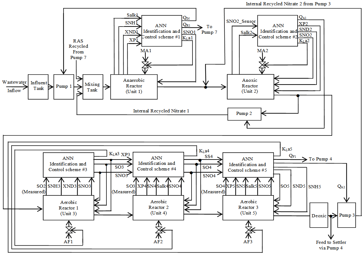Figure 4. The multivariable neural network-based NNARMAX model identification scheme for the five biological reactors of the AS-WWTP with the proposed manipulated inputs and controlled outputs

3). First Aerobic Reactor (Unit 3)

The objective here is to regulate XP3 = 449 g.m^-3, SO3 = 2 g.m^-3 and SNO3 = 6.2 g.m^-1 by manipulating the aeration intensity (K_La3 = 10 hr^-1 using SO2 (measured), SNH3, XND3, and SNO3 as inputs.

4). Second Aerobic Reactor (Unit 4)

The objective here is to regulate SO4 = 2 g.m^-3, SNO4 = 11.6 g.m^-1 and SS4 = 35 g.m^-3 by manipulating K_La4 = 10 hr^-1 using SO3 (measured), XP4, SN4, Salk4, and SNO4 as inputs.

5). Third Aerobic Reactor (Unit 5)

The objective here is to regulate SNH5 = 35 g.m^-3, SND5 = 13.5 g.m^-1, SO5 = 2 g.m^-3 by manipulating the internal recycled nitrate 2 (Q_A2 = 16485 m³.d^-1), feed flow rate (Q_F1 = 36892 m³.d^-1) depending on the feed flow decision system, and the aeration intensity (K_La5 = 3.5 hr^-1) using SO4 (measured), XP5, SN5, Salk5, and SNO5 as inputs.

4.2. Formulation of the AS-WWTP Model Identification Problem

4.2.1. Statement of the AS-WWTP Neural Network Model Identification Problem

The activated sludge wastewater treatment plant model defined by the benchmark simulation model no. 1 (BSM1) is described by eight coupled nonlinear differential equations given in Appendix A. The BSM1 model consist of thirteen states defined in Table 1 as follows: , , , , , , , , , , , , and out of which four states are measurable namely: (readily biodegradable substrate), (active heterotrophic biomass), (oxygen) and (nitrate and nitrite nitrogen). An additional important parameter is used to assess the amount of soluble solids in all the reactors including aerobic reactor of Unit 5.

As highlighted above, the main objective here is on the efficient neural network model identification to obtain a multivariable NNARMAX model equivalent of the activated sludge wastewater treatment plant (AS-WWTP) with a view in using the obtained model for multivariable adaptive predictive control of the AS-WWTP process in our future work. Thus, from Section 2, the measured inputs that influence the behaviour of the AS-WWTP process shown in Fig. 5 are:

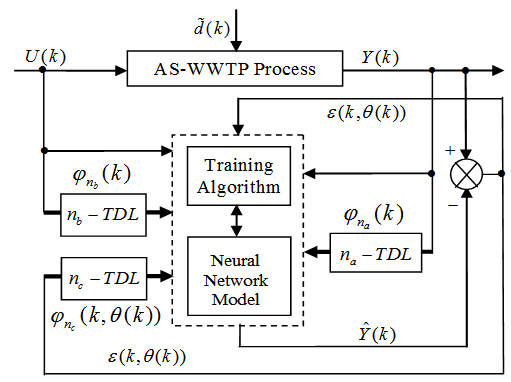Figure 5. The neural network model identification scheme for AS-WWTP based on NNARMAX model

(28)

From the arguments in Section 2, the output parameters that capture the behaviour of the AS-WWTP are defined here as:

(29)

Although, the multivariable system is formulated as 26–input 23–output control problem, but the neural network model identification is a much more complicated multiple–input multiple–output (MIMO) problem since all the fourteen states must be predicted at each sampling instant in order to obtain a reasonable approximate model that describes and captures the system’s dynamics at that instant. Thus, making the total outputs 37. Additional complexity arises from the number of past inputs and outputs in the regression matrix that defines the system. The neural network identification scheme used here is shown in Fig. 5 and is based on the NNARMAX model predictor discussed in Section 3. The input vector to the neural network (NN) consists of the regression vectors which are concatenated into for the NNARMAX models predictors discussed in Section 4 and defined here as follows:

(30)

(31)

(32)

(33)

The outputs of the neural network for the AS-WWTP process are the predicted values of the thirteen states together with the amount of total soluble solids (TSS), thus resulting in fourteen states to be predicted at each sampling instant given by:

(34)

Since disturbances play an important role in the evaluation of controller performances, three influent disturbance data are defined for different weather conditions, namely: dry-weather data, rain weather data, and storm weather data. The data for these three influent disturbances are provided by the European COST Actions for evaluating controller performances [27]–[29]. In this study, the dry weather influent data is used in order to measure how well the trained neural network mimic the dynamics of the AS-WWTP process to meet the control requirement specified above. The dry weather data contains two weeks of influent data at 15 minutes sampling interval. Although, disturbances affecting the AS-WWTP are incorporated into dry-weather data provided by the COST Action Group, additional sinusoidal disturbances with non-smooth nonlinearities are introduced in the last sub-section of this section to further investigate the closed-loop controllers’ performances based on an updated neural network model at each sampling time instants.

4.2.2. Experiment with the BSM1 for AS-WWTP Process Neural Network Training Data Acquisition

For the efficient control of the activated sludge wastewater treatment plant (AS-WWTP) using neural network, a neural network (NN) model of the AS-WWTP process is needed which requires that the NN be trained with dynamic data obtained from the AS-WWTP process. In other to obtain dynamic data for the NN training, the validated and generally accepted COST Actions 624 benchmark simulation model no. 1 (BSM1) is implemented and simulated using MATLAB and Simulink as shown in Fig. 6. The BSM1 process model for the AS-WWTP process is given in Appendix A.

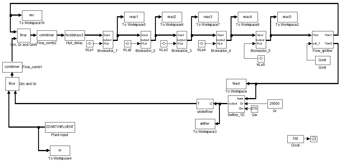Figure 6. Open-loop steady-state benchmark simulation model No.1 (BSM1) with constant influent

A two-step simulation procedure defined in the simulation benchmark [27]–[29] is used in this study. The first step is the steady state simulation using the constant influent flow (CONSTINFLUENT) for 150 days as shown and implemented in Fig. 6. Note that each simulation sample period indicated by the “Clock” of the AS-WWTP Simulink model in Fig. 6 corresponds to one day. In the second step, starting from the steady state solution obtained with the CONSTINFLUENT data and using the dry-weather influent weather data (DRYINFLUENT) as inputs, the AS-WWTP process is then simulated for 14 days using the same Simulink model of Fig. 6 but by replacing the CONSTINFLUENT influent data with the DRYINFLUENT influent data. This second simulation generates 1345 dynamic data in which is used for NN training while the 130first day dry-weather data samples provided by the COST Actions 624 and 682 is used for the trained NN validation.

4.2.3. The Incremental or Online Back-Propagation (INCBP) Algorithm

In order to investigate the performance of the ARLS, the so-called incremental (or online) back-propagation (INCBP) algorithm is used to this purpose. The incremental or online back-propagation (INCBP) algorithm was originally proposed by [38] which has been modified in [27] is used in this paper. The incremental back-propagation (INCBP) algorithm is easily derived by setting the covariance matrix on the left hand side of (20) in Section 3.3.1under the formulation of the ARLS algorithm; that is:

(35)

where is the step size and is an identity matrix of appropriate dimension. Next, the basic back-propagation given from [27] as:

(36)

is used to update the algorithm in (35). Finally, all that is required is to specify a suitable step size and carry out the recursive computation of the gradient given by (36).

4.2.4. Scaling the Training Data and Rescaling the Trained Network that Models the AS-WWTP Process

Due to the fact the input and outputs of a process may, in general, have different physical units and magnitudes; the scaling of all signals to the same variance is necessary to prevent signals of largest magnitudes from dominating the identified model. Moreover, scaling improves the numerical robustness of the training algorithm, leads to faster convergence and gives better models. The training data are scaled to unit variance using their mean values and standard deviations according to the following equations:

(37)

where and , are the mean and standard deviation of the input and output training data pair; and and are the scaled inputs and outputs respectively. Also, after the network training, the joint weights are rescaled according to the expression

(38)

so that the trained network can work with other unscaled validation data and test data not used for training. However, for notational convenience, and shall be used.

4.2.5. Training the Neural Network that Models the Biological Reactors of the AS-WWTP Process

The NN input vector to the neural network (NN) is the NNARMAX model regression vector defined by (33). The input , that is the initial error estimates given by (32), is not known in advance and it is initialized to small positive random matrix of dimension by. The outputs of the NN are the predicted values of given by (34).

For assessing the convergence performance, the network was trained for = 100 epochs (number of iterations) with the following selected parameters: , , , , , (NNARMAX), , , and . The details of these parameters are discussed in Section 3; where and are the number of inputs and outputs of the system, and are the orders of the regressors in terms of the past values, is the total number of regressors (that is, the total number of inputs to the network), and are the number of hidden and output layers neurons, and and are the hidden and output layers weight decay terms. The four design parameters for adaptive recursive least squares (ARLS) algorithm defined in (22) are selected to be: α=0.5, β=5e-3, =1e-5 and π=0.99 resulting to γ=0.0101. The initial values for ē_min and ē_max in (23) are equal to 0.0102 and 1.0106e+3 respectively and were evaluated using (23). Thus, the ratio of ē_min/ē_max from (23) is 9.9018e+4 which imply that the parameters are well selected. Also, is selected to initialize the INCBP algorithm given in (36).

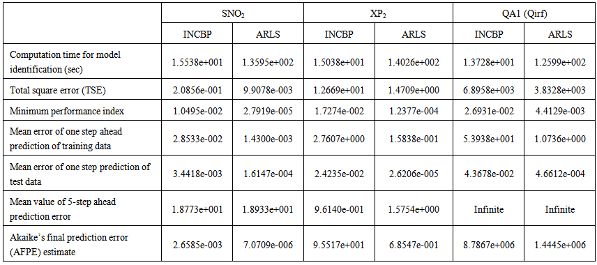
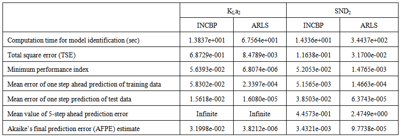
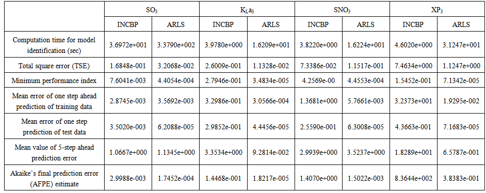
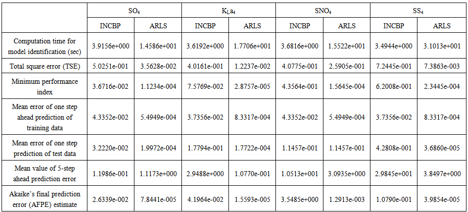
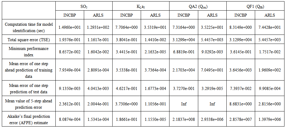
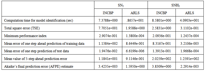
The 1345 dry-weather training data is first scaled using equation (37) and the network is trained for epochs using the proposed adaptive recursive least squares (ARLS) and the incremental back-propagation (INCBP) algorithms proposed in Sections 3.3 and 4.2.3. After network training, the trained network is again rescaled respectively according to (38), so that the resulting network can work or be used with unscaled AS-WWTP data. Although, the convergence curves of the INCBP and the ARLS algorithms for 100 epochs each are not shown but the minimum performance indexes for both algorithms are given in the third rows of Tables 4, 5, 6, 7 and 8 for the five reactors. As one can observe from these Tables, the ARLS has smaller performance index when compared to the INCBP which is an indication of good convergence property of the ARLS at the expense of higher computation time when compared the small computation time used by the INCBP for 100 epochs as evident in the first rows of Tables 4, 5, 6, 7 and 8.

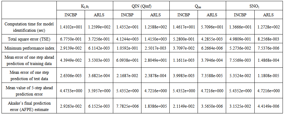Table 4. Anaerobic reactor (Unit 1)

Table 5(a). Anoxic reactor (Unit 2)

Table 5(b). Anoxic reactor (Unit 2)

Table 6. First aerobic reactor (Unit 3)

Table 7. Second aerobic reactor (Unit 4)

Table 8(a). Third aerobic reactor (Unit 5)

Table 8(b). Third aerobic reactor (Unit 5)

The total square error (TSE) discussed in subsection 3.1, for the network trained with the INCBP and the ARLS algorithms are given in the second rows of Table 4, 5, 6, 7 and 8. Again, the ARLS algorithm also has smaller mean square errors and minimum performance indices when compared to the INCBP algorithm. The small values of the mean square error (MSE) and the minimum performance indices indicate that ARLS performs better than the INCBP for the same number of iterations (epochs). These small errors suggest that the ARLS model approximates better the AS-WWTP process giving smaller errors than the INCBP model.

4.3. Validation of the Trained NNARMAX Model of the AS-WWTP Process

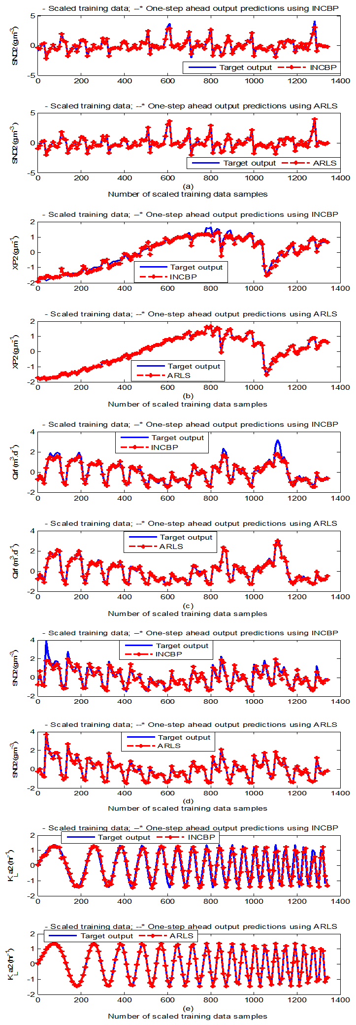
According to the discussion on network validation in Section 3.4, a trained network can be used to model a process once it is validated and accepted, that is, the network demonstrates its ability to predict correctly both the data that were used for its training and other data that were not used during training. The network trained by the INCBP and the proposed ARLS algorithms has been validated with three different methods by the use of scaled and unscaled training data as well as with the 130 dry-weather data reserved for the validation of the trained network for the AS-WWTP process.

The results shown in Fig. 7, Fig. 8 and Fig. 9 each having (a) to (e) corresponds to the five reactors respectively. The output parameters obtained in each of (a) to (e) were previously defined during the problem formulation in Section 4.2.1 but they are redefined here again as they appear in the next few figures (Fig. 7, Fig. 8 and Fig. 9) as follows:

(a) is for the anaerobic reactor (Unit 1) for the nitrate concentration SNO₁ in g.m^-3, the influent flow rate Q_IN (Qinf) in m³.d^-1, the RAS recycle flow rate Q_R1 (Q_ras) in m³.d^-1, and the aeration intensity K_La1 = 1 hr^-1.

(b) is for the anoxic reactor (Unit 2) for nitrate and nitrite nitrogen SNO2 in g.m^-1, particulate products arising from biomass decay XP2 in g.m^-1, internal recycled nitrate 1 flow rate Q_A1 (Qirf) in m³.d^-1), soluble biodegradable organic nitrogen SND2 in g/m³ and the aeration intensity K_La2 in hr^-1.

(c) is for the first aerobic reactor (Unit 3) for particulate product arising from biomass decay XP3 in g.m^-3, soluble oxygen SO3 in g.m^-3 and nitrate and nitrite nitrogen SNO3 in g.m^-1 and the aeration intensity K_La3 in hr^-1.

(d) is for the second aerobic reactor (Unit 4) for readily biodegradable substrate SS4 in g.m^-3, soluble oxygen SO4 in g.m^-3, nitrate and nitrite nitrogen SNO4 in g.m^-1 and the aeration intensity K_La4 in hr^-.

(e) is for third aerobic reactor (Unit 5) for ammonia and ammonium nitrogen SNH5 in g.m^-3, soluble biodegradable organic nitrogen SND5 in g.m^-1, soluble oxygen SO5 in g.m^-3, the internal recycled nitrate 2 flow rate Q_A2 (Qirn) in m³.d^-1, feed flow rate Q_F1 (Qffr) in m³.d^-1 and the aeration intensity K_La5 in hr^-1.

4.3.1. Validation by the One-Step Ahead Predictions Simulation

In the one-step ahead prediction method, the errors obtained from one-step ahead output predictions of the trained network are assessed. In Fig. 7(a)–(e) the graphs for the one-step ahead predictions of the scaled training data (blue -) against the trained network output predictions (red --*) using the neural network models trained by INCBP and ARLS algorithms respectively are shown for 100 epochs.

The mean value of the one-step ahead prediction errors are given in the fourth rows of Table 4, 5, 6, 7 and 8 respectively. It can be seen in the figures that the network predictions of the training data closely match the original training data. Although, the scaled training data prediction errors by both algorithms are small, the ARLS algorithm appears to have a much smaller error when compared to the INCBP algorithm as shown in the fourth rows of Table 4 to 8. These small one-step ahead prediction errors are indications that the networks trained using the ARLS captures and approximate the nonlinear dynamics of the five reactors of the AS-WWTP process to a high degree of accuracy. This is further justified by the small mean values of the TSE obtained for the networks trained using the proposed ARLS algorithms for the process as shown in the second rows of Table 4 to Table 8.

Furthermore, the suitability of the INCBP and the proposed ARLS algorithms for neural network model identification for use in the real AS-WWTP industrial environment is investigated by validating the trained network with the 130 unscaled dynamic data obtained for dry-weather as provided by the COST Action Group. Graphs of the trained network predictions (red --*) of the validation (test) data with the actual validation data (blue -) using the INCBP and the proposed ARLS algorithms are shown in Fig. 8(a)–(e) for the five reactors of the AS-WWTP process based on the selected process parameters. The almost identical prediction of these data proves the effectiveness of the proposed approaches. The prediction accuracies of the unscaled test data by the networks trained using the INCBP and the proposed ARLS algorithm evaluated by the computed mean prediction errors shown in the fifth rows of Table 4 to Table 8. Again, one can observe that although the validation data prediction errors obtained by both algorithms are small, the validation data predictions errors obtained with the model trained by the proposed ARLS algorithm appears much smaller when compared to those obtained by the model trained using the INCBP algorithm. These predictions of the unscaled validation data given in Fig. 8(a)–(e) as well as the mean value of the one step ahead validation (test) prediction errors in the fifth rows of Tables 4, 5, 6, 7 and 8 verifies the neural network ability to model accurately the dynamics of the five reactors of the AS-WWTP process based on the dry-weather influent data using the proposed ARLS training algorithm.

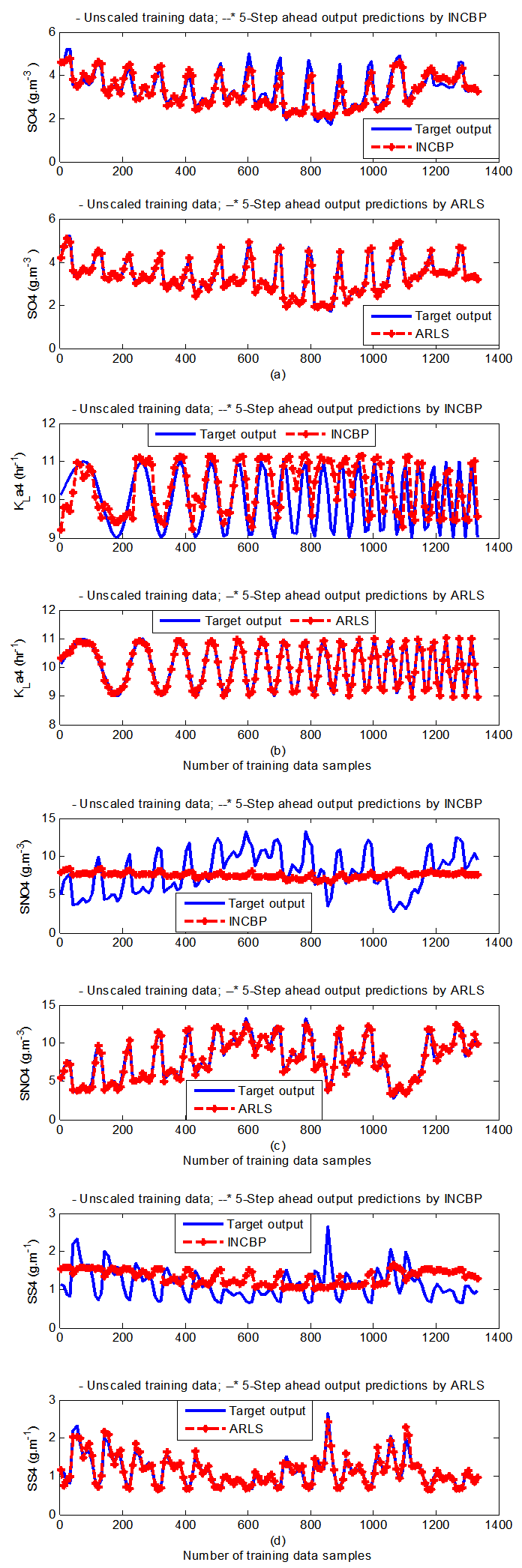
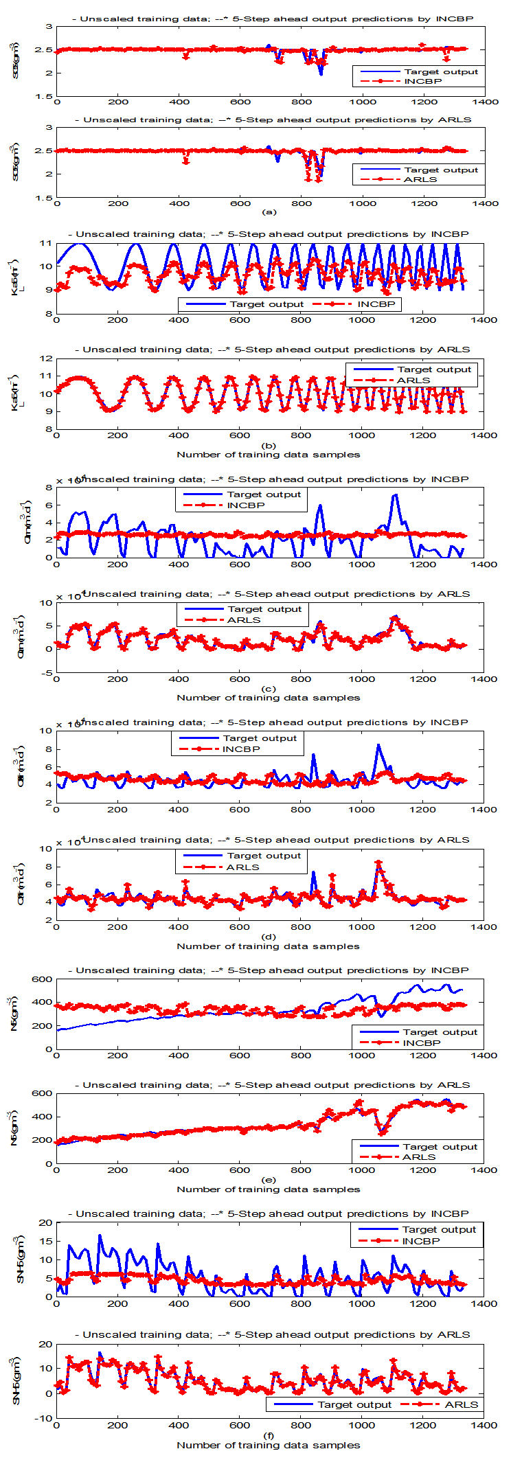
4.3.2. K–Step Ahead Prediction Simulations for the AS-WWTP Process

The results of the K-step ahead output predictions (red --*) using the K-step ahead prediction validation method discussed in Section 3.4 for 5-step ahead output predictions (K = 5) compared with the unscaled training data (blue -) are shown in Fig. 9(a) to Fig. 9(e) for the networks trained using the INCBP and the proposed ARLS. Again, the value K = 5 is chosen since it is a typical value used in most model predictive control (MPC) applications. The comparison of the 5-step ahead output predictions performance by the network trained using the INCBP and the proposed ARLS algorithms indicate the superiority of the proposed ARLS over the so-called INCBP algorithm.

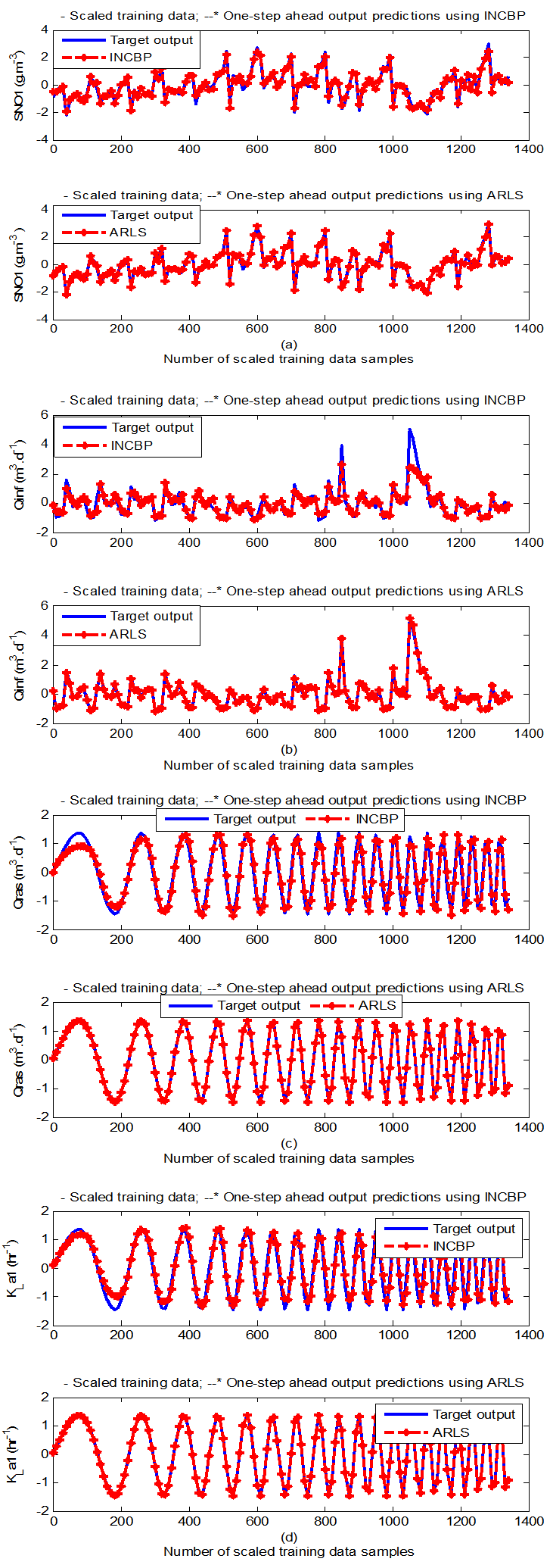Figure 7(a). One-step ahead prediction of scaled SNO1, QIN (Qinf), QR1 (Qras) and KLa1 training data

Figure 7(b). One-step ahead prediction of scaled SNO2, XP2, QA1 (Qirf), SND2 and KLa2 training data

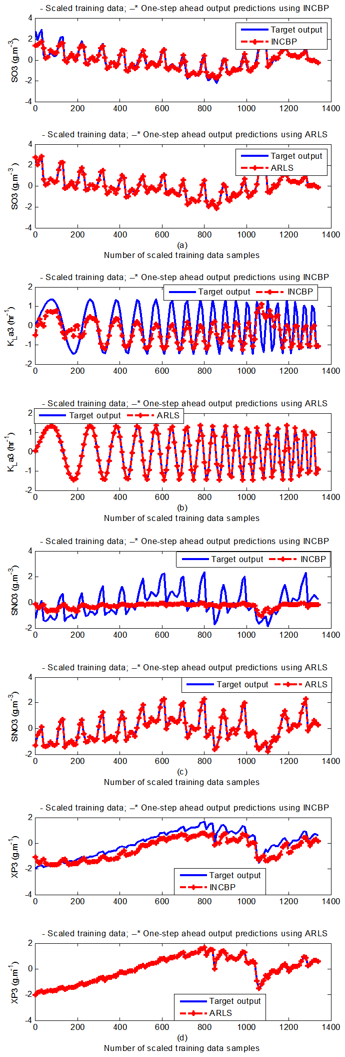Figure 7(c). One-step ahead prediction of scaled SO3, KLa3, SNO3 and XP3 training data

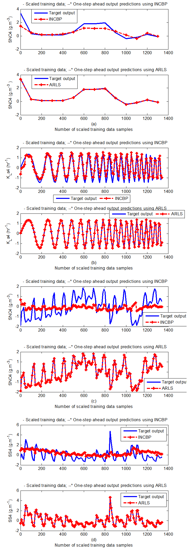Figure 7(d). One-step ahead prediction of scaled SO4, KLa4, SNO4 and SS4 training data

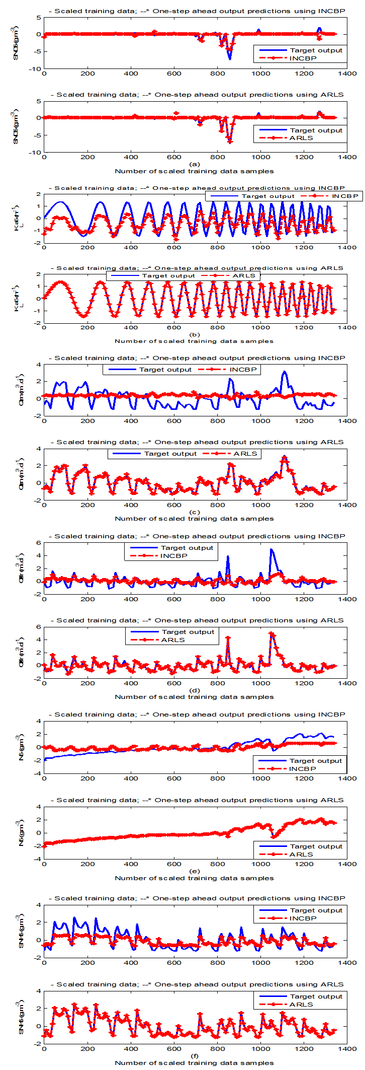Figure 7(e). One-step ahead prediction of scaled SO5, KLa5, QA2 (Qirn), QF1 (Qffr), SND5 and SNH5 training data

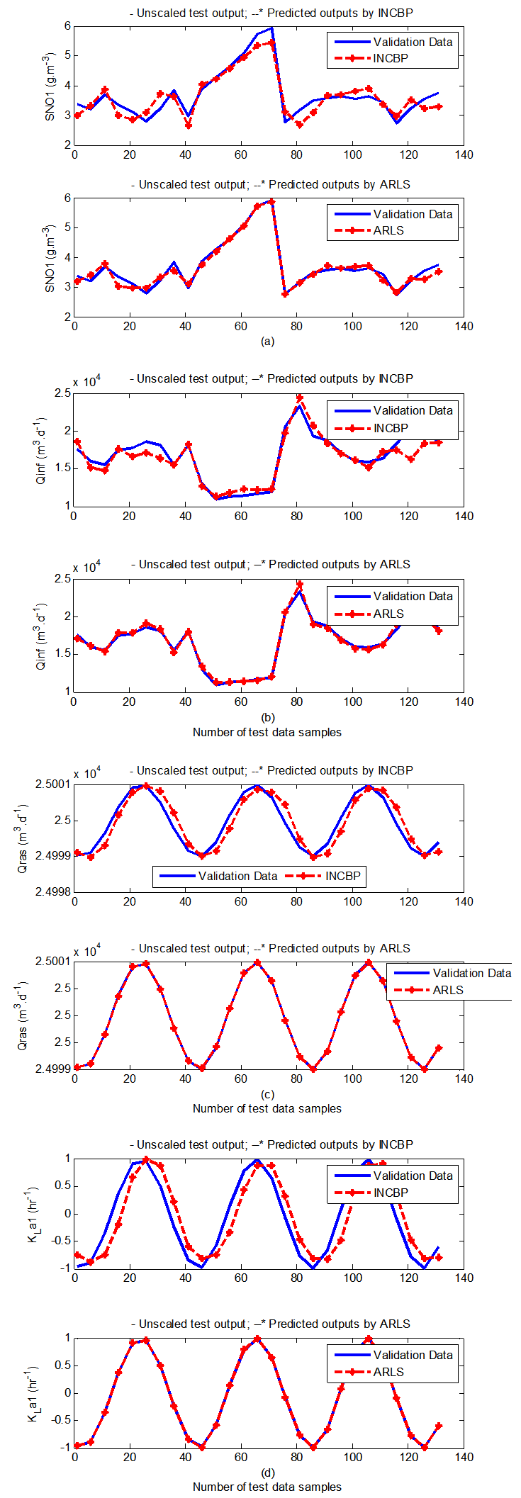Figure 8(a). One-step ahead prediction of unscaled SNO1, QIN (Qinf), QR1 (Qras) and KLa1 validation data

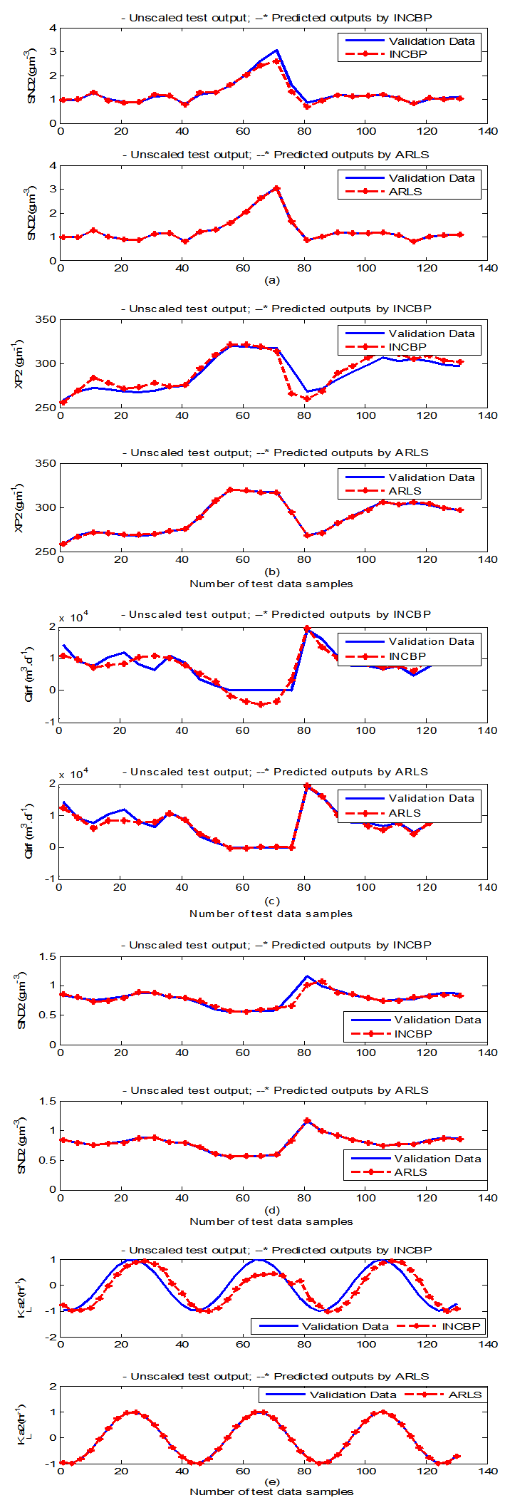Figure 8(b). One-step ahead prediction of unscaled SNO2, XP2, QA1 (Qirf), SND2 and KLa2 validation data

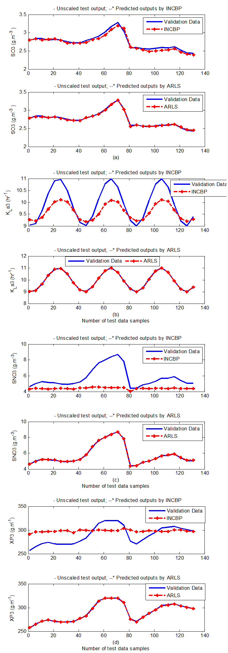Figure 8(c). One-step ahead prediction of unscaled SO3, KLa3, SNO3 and XP3 validation data

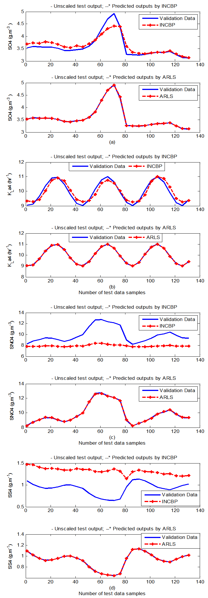Figure 8(d). One-step ahead prediction of unscaled SO4, KLa4, SNO4 and SS4 validation data

Figure 8(e). One-step ahead prediction of unscaled SO5, KLa5, QA2 (Qirn), QF1 (Qffr), SND5 and SNH5 validation data

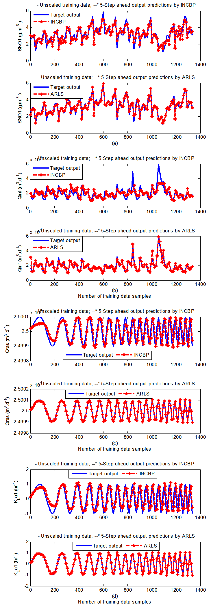Figure 9(a). 5-step ahead prediction of unscaled SNO1, QIN (Qinf), QR1 (Qras) and KLa1 training data

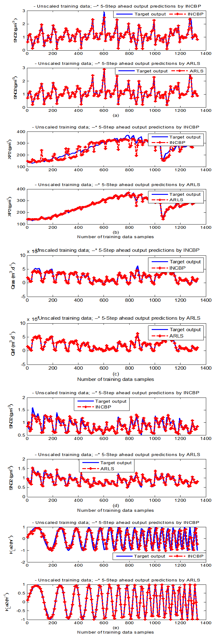Figure 9(b). 5-step ahead prediction of unscaled SNO2, XP2, QA1 (Qirf), SND2 and KLa2 training data

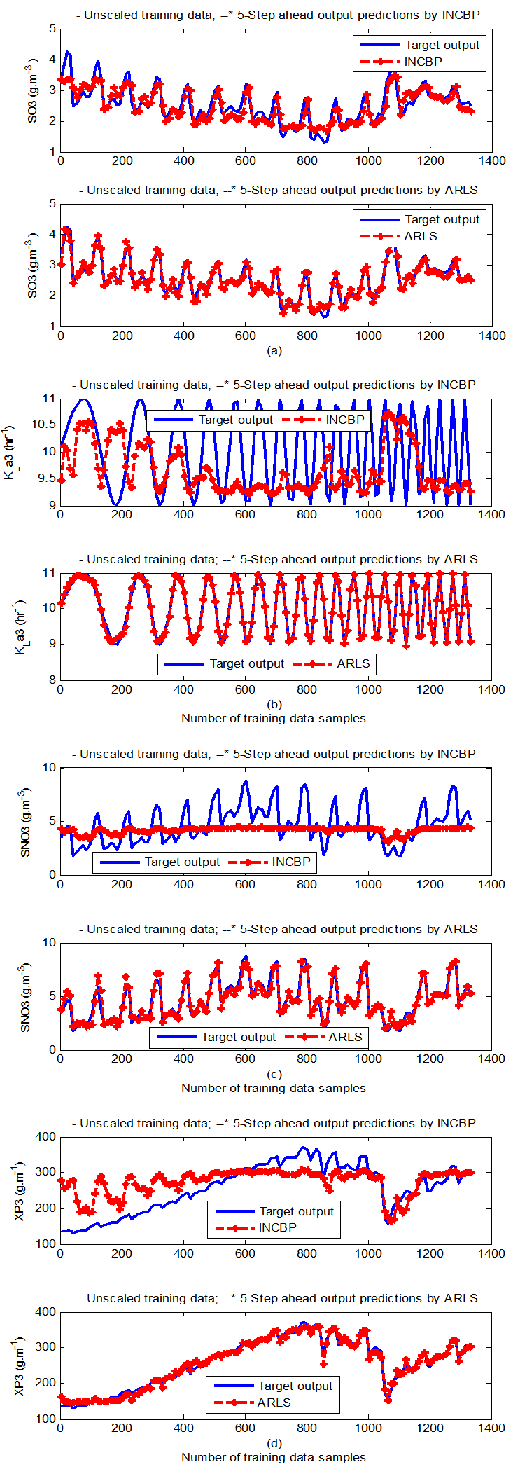Figure 9(c). 5--step ahead prediction of unscaled SO3, KLa3, SNO3 and XP3training data

Figure 9(d). 5-step ahead prediction of unscaled SO4, KLa4, SNO4 and SS4 training data

Figure 9(e). 5-step ahead prediction of unscaled SO5, KLa5, QA2 (Qirn), QF1 (Qffr), SND5 and SNH5 training data

The computation of the mean value of the K-step ahead prediction error (MVPE) using (27) is given in the sixth rows of Tables 4, 5, 6, 7 and 8 by the network trained using INCBP and the proposed ARLS algorithms respectively. The small mean values of the 5-step ahead prediction error (MVPE) are indications that the trained network approximates the dynamics of the five reactors of the AS-WWTP process to a high degree of accuracy with the networks of both algorithms but with the network based on the ARLS algorithm giving much smaller distant prediction errors.

4.3.3. Akaike’s Final Prediction Error (AFPE) Estimates for the AS-WWTP Process

The implementation of the AFPE algorithm discussed in Section 3.4 and defined by (25) for the regularized criterion for the network trained using the INCBP and the proposed ARLS algorithms with multiple weight decay gives their respective AFPE estimates which are defined in the seventh rows of Tables 4, 5, 6, 7 and 8 respectively. These relatively small values of the AFPE estimate indicate that the trained networks capture the underlying dynamics of the aerobic reactor of the AS-WWTP and that the network is not over-trained [34]. This in turn implies that optimal network parameters have been selected including the weight decay parameters. Again, the results of the AFPE estimates computed for the networks trained using the proposed ARLS algorithm are much smaller when compared to those obtained using INCBP algorithm.

5. Conclusions

This paper presents the formulation of an advanced online nonlinear adaptive recursive least squares (ARLS) model identification algorithm based on artificial neural networks for the nonlinear model identification of a AS-ASWWTP process. The mathematical model of the process obtained from COST Actions 632 and 624 has been simulated in open-loop to generate the training data while the First Day data, also provided by the COST Actions group, is used as the validation (test) data. In order to investigate the performance of the proposed ARLS algorithm, the incremental backpropagation (INCBP), which is also an online algorithm, is implemented and compared with proposed ARLS. The results from the application of these algorithms to the modeling of the five units of the AS-WWTP biological reactors as well as the validation results show that the neural network-based ARLS outperforms the INCBP algorithm with much smaller predictions error and good tracking abilities with high degree of accuracy and that the proposed ARLS model identification algorithm can be used for the AS-ASWWTP process in an industrial environment.

The next aspect of the work is on the dynamic modelling and nonlinear model identification of the multivariable NNARMAX model of the secondary settler and the clarifier as well as effluent tank to complete the modelling of the AS-WWTP process. As a future work, the development of an adaptive fuzzy rule-based logic decision system which would be able produce the set points that can be used for the development of an intelligent multivariable nonlinear adaptive model-based predictive control algorithm for the efficient control of the complete AS-WWTP by manipulating the pumps based on some decision parameters could be considered.

Appendix

Appendix A: AS-WWTP Process Model

As mentioned in above, the BSM1 model involves eight different chemical reactions incorporating thirteen different components [1], [27]–[29]. These components are classified into soluble components and particulate components. The nomenclatures and parameter definitions used for describing the AS-WWTP in this work are given in Table 1. The Moreover, four fundamental processes are considered: the growth and decay of biomass (heterotrophic and autotrophic), ammonification of organic nitrogen and the hydrolysis of particulate organics. The typical schematic of the AS-WWTP is shown in Fig. 1.

Table A1. Stiochiometric parameters with their units and values

The eight basic processes that are used to describe the biological behaviour of the AS-WWTP process are:

: Aerobic growth of heterotrophs

(A.1)

: Anoic growth of heterotrophs

(A.2)

: Aerobic growth of autotrophs

(A.3)

: Decay of heterotrophs

(A.4)

: Decay of autotrophs

(A.5)

: Ammonification of soluble organic nitrogen

(A.6)

: Hydrolysis of entrapped organics

(A.7)

: Hydrolysis of entrapped organic nitrogen

(A.8)

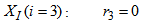
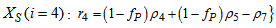
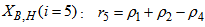
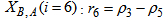
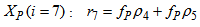
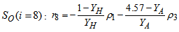
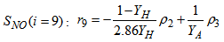
The observed thirteen conversion rates result from combinations of basic processes (A.1) to (A.8) as follows:

(A.9)

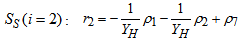(A.10)

(A.11)

(A.12)

(A.13)

(A.14)

(A.15)

(A.16)

(A.17)

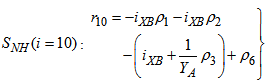(A.18)

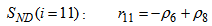(A.19)

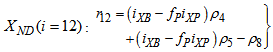(A.20)

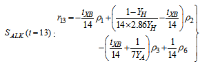(A.21)

The biological parameter values used in the BSM1 correspond approximately to a temperature of 15°C. The stiochiometric parameters are listed in Table A.1 and the kinetic parameters are listed in Table A.2.

Table A2. Kinetic parameters with their units and values

Appendix B: General Characteristics of the Biological Reactors

As shown in Fig. 1, the general characteristics of the biological reactors for the default case are five compartments where the first two (Unit 1 and Unit 2) are non-aerated compartments whereas the last three (Unit 3, Unit 4 and Unit 5) are aerated compartments.

Unit 3 and Unit 4 of the aerated compartments have a fixed oxygen transfer coefficient of . In Unit 5, the dissolved oxygen (DO) concentration is controlled at a level of by manipulation of the. Each of the five compartments has a flow rate, the concentration, and the reaction rate; where is the number of compartments. The volume of the non-aerated compartments is each while the volume of the aerated compartments is.

The general equation for the reactor mass balances is given as:

For (Unit 1)

(B.1)

(B.2)

For to (Unit 2, Unit3, Unit 4 and Unit 5)

(B.3)

(B.4)

Special case for oxygen:

(B.5)

where the saturation concentration for oxygen is. Also,

(B.6)

(B.7)

(B.8)

(B.9)