-
Paper Information
- Previous Paper
- Paper Submission
-
Journal Information
- About This Journal
- Editorial Board
- Current Issue
- Archive
- Author Guidelines
- Contact Us
American Journal of Intelligent Systems
p-ISSN: 2165-8978 e-ISSN: 2165-8994
2014; 4(1): 15-19
doi:10.5923/j.ajis.20140401.03
An Investigation of Differencing Effect in Multiplicative Neuron Model Artificial Neural Network for Istanbul Stock Exchange Time Series Forecasting
 Abstract
 Reference
 Full-Text PDF
 Full-text HTML
Ali Zafer Dalar1, Erol Eğrioğlu1, Ufuk Yolcu2, Damla İlter3, Özge Gündoğdu4
1Department of Statistics, Ondokuz Mayis University, Samsun, 55139, Turkey
2Department of Statistics, Ankara University, Ankara, 06100, Turkey
3Department of Statistics, Mimar Sinan Fine Arts University, Istanbul, 34349, Turkey
4Department of Econometrics, Cumhuriyet University, Sivas, 58140, Turkey
Correspondence to: Erol Eğrioğlu, Department of Statistics, Ondokuz Mayis University, Samsun, 55139, Turkey.
| Email: |  |
Copyright © 2012 Scientific & Academic Publishing. All Rights Reserved.
In recent years, good alternative methods have been proposed to obtain forecasts for a time series. Artificial neural networks have been commonly used for forecasting purpose in the literature. Although, multilayer perceptron artificial neural network is the most used artificial neural network type, multiplicative neuron model artificial neural networks have been used to obtain forecasts for six years. In the literature, many studies used original series without applying any differencing operation. Thereby, non-stationary time series were used in the artificial neural networks. It is very difficult to find appropriate time series model for non-stationary time series in probabilistic time series methods. Similarly, differencing can be useful obtaining forecasts by artificial neural networks. Differencing effect has not been sufficiently discussed for artificial neural networks. It has not been discussed for multiplicative neuron model artificial network in the literature, yet. Aim of this study is discussing of differencing effect for multiplicative neuron model artificial neural networks. Istanbul stock exchange data (IEX) sets were used to explore differencing effect. The data setsare made up of five time series for years between 2009 and 2013. All of time series were daily observed and observations of them are taken for first five months. It is shown that differencing operation is not useful for forecasting IEX as a result of statistical hypothesis tests.
Keywords: Artificial Neural Network, Difference Operator, Forecasting, Multiplicative Neuron Model, Particle Swarm Optimization, Artificial Bee Colony Optimization
Cite this paper: Ali Zafer Dalar, Erol Eğrioğlu, Ufuk Yolcu, Damla İlter, Özge Gündoğdu, An Investigation of Differencing Effect in Multiplicative Neuron Model Artificial Neural Network for Istanbul Stock Exchange Time Series Forecasting, American Journal of Intelligent Systems, Vol. 4 No. 1, 2014, pp. 15-19. doi: 10.5923/j.ajis.20140401.03.
1. Introduction
- Forecasting is the process of making statements about events whose actual outcomes have not yet been observed. Forecasting methods can be classified into two classes as probabilistic and non-probabilistic methods. Artificial neural networks are non-probabilistic methods. Because artificial neural networks do not need strict assumptions such as normality, linearity, they have been commonly used in the literature in recent years.Zhang et al. (1998) and Hippert et al. (2001) are good surveys of literature about neural network forecasting methods. In the literature, many of papers asserted that neural networks are outperforms traditional forecasting methods like autoregressive moving average (ARMA) models. Multilayer perceptron neural networks have been commonly used for obtaining forecasts. Alpaslan et al.(2012) statistically investigated some important factors to obtain more accurate forecasts by using multilayer perceptron neural networks.Aladag et al. (2012), Cagcag (2013) and Oner et al. (2013) proposed hybrid methods which are based on multilayer perceptron neural networks. In recent years, different kinds of artificial neural network models have been proposed for forecasting. Yadav et al. (2007) introduced multiplicative neuron model ANN (MNM-ANN) which has only one neuron in the hidden layer. Because MNM-ANN has one neuron, determining number of hidden layer neurons is not needed. This is very important, because determining number of hidden layer neurons is important problem for multilayer perceptron. Zhaou andYang (2009) and Samanta (2011) used particle swarm optimization method to train MNM-ANN. Particle swarm optimization has been used different aim in Itamiya et al. (2013). There are two modifications of multiplicative neuron model artificial network in literature. Yolcu et al. (2013) and Aladag et al. (2013) proposed different artificial neural networks which are employed multiplicative neuron model.Egrioglu et al. (2013) used multiplicative neuron model in a fuzzy time series forecasting algorithm.Stationarity of time series is discussable assumption in the practical application of ANN for forecasting. In the literature, many authors don’t take into account stationarity of time series. There are some papers in which stationary assumption are investigated. It is shown that first order differencing is useful for forecasting with ANN in Chow and Leung (1996). Kim et al. (2004) investigated whether it is feasible to relax the stationarity condition to non-stationary time series. Ghazali et al. (2011) put forward that ANN can produce accurate forecasts for non-stationary time series. Kandananond (2013) found that multilayer perceptron ANN is better than support vector machine ANN for stationary time series. Stationary assumption has not been investigated for MNM-ANN in the literature, yet. In this paper, differencing effect is investigated for MNM-ANN by using statistical hypothesis tests. In the second section, MNM-ANN and its training algorithm are briefly given. Experimental study is summarized in section three. In the fourth section, conclusions are given and they are discussed.
2. MNM-ANN
- Yadav et al. (2007) was firstly proposed MNM-ANN. The architecture of MNM-ANN is given Fig. 1.
 are inputs of MNM-ANN.
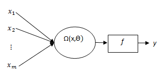 | Figure 1. Architecture of MNM-ANN |
 is aggregation function and it has multiplicative structure. In MNM-ANN architecture, there is only one neuron and its output is calculated as below:
 | (1) |
 and
and  are weight and bias for ith input, respectively. The activation function
  was selected as logistic activation function in Yadav et al. (2007). The logistic activation function can be given as follow:
 | (2) |
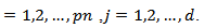
 . Although Yadav et al. (2007) utilized back propagation algorithm for training MNM-ANN, it can be performed by using particle swarm optimization. Zhaou and Yang (2009), Samanta (2011) Yolcu et al. (2013) and Aladag et al. (2013) used particle swarm optimization to train multiplicative neuron based neural network. Alpaslan et al. (2014) used artificial bee colony algorithm to train MNM-ANN.Particle swarm optimization (PSO) was firstly proposed in Kennedy and Eberhart (1995). The PSO algorithm for training MNM-ANN is given below. Algorithm 1. PSO algorithm used to train the proposed MNM-ANN modelStep 1. Positionsand velocities of each mth (m = 1,2, …, pn) particles are randomly determined and kept in vectors Pm and Vm given as follows:
 | (3) |
 | (4) |
 represents jth position of mth particle. pn and d represents the number of particles in a swarm and positions, respectively. The initial positions and velocities of each particle in a swarm are randomly generated from uniform distribution (0,1) and (-vm,vm), respectively. Positions of a particle are consisted from weights and biases. Each particle gives a solution set for the neural network.Step 2. The parameters of PSO are determined.In the first step, the parameters which direct the PSO algorithm are determined. These parameters are pn, vm,c1i, c1f, c2i, c2f, w1, and w2. Let c1 and c2 represents cognitive and social coefficients, respectively, and w is the inertia parameter. Let (c1i, c1f), (c2i, c2f), and (w1, w2) be the intervals which includes possible values for c1, c2 and w, respectively. At each iteration, these parameters are calculated by using the formulas given in (5), (6) and (7).
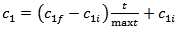 | (5) |
 | (6) |
 | (7) |
 | (8) |
 | (9) |
 | (10) |
 | (11) |
 | (12) |
 Step 7. The best solution is determined. The elements of Gbest are taken as the best weight values of the new ANN model.Artificial bee colony (ABC) algorithm was firstly introduced by Karaboga (2005). Karaboga et al. (2007) utilized ABC algorithm to train feed forward neural network. The ABC algorithm for training MNM-ANN is given below.Algorithm 2. ABCAlgorithm for training MNM-ANNStep 1. The number of food sources (SN) andlimitvalue are determined. Step 2. Initial food source locations are randomly generated from
  interval.Step 3. Fitness function values are calculated for each food source. Fitness function is MSE value that is calculated by using locations of the source. The locations of source can be used as weights and biases for MNM-ANN.Step 4. Sending employed bees to the food source locations.New food source
  is obtained by using (13). To calculate
  location, a neighbor source (kth) is randomly selected. The jth location of the new source is obtained from (13). Other locations of the new source are taken by ithsource.
 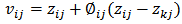 | (13) |
 | (14) |
 interval instead of the exhausted source. The failure counter is set to zero for the new source.Step 8. Stopping conditions are checked. If the stopping conditions are met, skip to step 9. Otherwise, back to step 4. Step 9. The best food source is taken as the solution.
3. Experimental Study
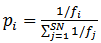
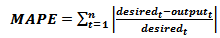
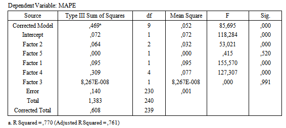
- In the experimental study, IEX data sets were used to test differencing effect. Details of data sets are given below:Set 1. BIST 100 data for IEX, it is daily observed between 02/01/2009 and 29/05/2009 dates.Set 2. BIST 100 data for IEX, it is daily observed between 04/01/2010 and 31/05/2010 dates.Set 3. BIST 100 data for IEX, it is daily observed between 03/01/2011 and 31/05/2011 dates.Set 4. BIST 100 data for IEX, it is daily observed between 02/01/2012 and 31/05/2012 dates.Set 5. BIST 100 data for IEX, it is daily observed between 02/01/2013 and 29/05/2013 dates.Firstly, Augmented Dickey Fuller (ADF) unit root test is applied for five series by using Eviews Package program. According to test results, all series have unit roots and first differences of all series are stationary time series. In the experimental study, all series and their first differences are solved by using MNM-ANN. In the application, three different test sets were used for all series. The data of test sets are obtained %10, %20 and %30 of all observations for all series. PSO and ABC algorithms were used to train MNM-ANN. Input numbers are taken 2,3,4 and 5. In the experimental design, all factors are listed below:Factor 1 is differencing operation. This factor has two levels which are differenced (1) and original series (2).Factor 2 is test set length. This factor has three levels. These levels are %10 (1), %20 (2) and %30 (3).Factor 3 is input numbers of MNM-ANN. Levels of the factor are 2 (1), 3 (2), 4 (3) and 5(4). There are four levels for this factor.Factor 4 is years. This factor has five levels which are 2009 (1), 2010 (2), 2011 (3), 2012 (4) and 2013 (5).Factor 5 is training algorithm. Levels are PSO (1) and ABC (2).Observations of dependent variable are mean absolute percentage error (MAPE) values which are obtained for test data sets in each run. MAPE can be calculated by using (15).
 | (15) |
|
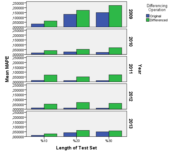 | Figure 2. Mean of MAPE values for the levels of Factor 1,2 and 4 |
4. Conclusions
- In this study, differencing effect for MLP-ANN are investigated. An experimental study was designed to test differencing effect. The obtained results are showed that there is no need to difference in MLP-ANN. MLP-ANN can give better results for original and non-stationary time series. These conclusions are obtained for IEX data. It is clear that the different results can be obtained for different data sets. According to obtained results, it can be asserted that IEX time series can be solved with MLP-ANN by using their original data. Thus, stationary is not needed and it is not strict assumption of MLP-ANN for IEX time series. In the future studies, the similar experimental study can be applied for exchange data sets of other countries. The results may generalize for stock exchange data sets.