Akihiko Kawashima1, Yasuo Sugai2
1Graduate School of Engineering, Nagoya University, Nagoya, Japan
2Graduate School of Engineering, Chiba University, Chiba, Japan
Correspondence to: Akihiko Kawashima, Graduate School of Engineering, Nagoya University, Nagoya, Japan.
| Email: |  |
Copyright © 2012 Scientific & Academic Publishing. All Rights Reserved.
Abstract
In the study of Traveling Salesman Problem (TSP), a main theme is the reduction of computational cost. This reduction needs the intelligence which is heuristics or the theoretical knowledge such as necessary conditions for optimality. If TSP can be manipulated as classification problems, the analysis of the classifier, which can solve efficiently these classification problems, provides the required intelligence. In fact, we can replace the TSP with a classification problem and some Shortest Hamiltonian Path Problems (SHPPs) which also can be replaced with these sub problems in the same way. Hence, the TSPs are equivalent to the classification problems. In this paper, we propose the theoretical framework to solve the TSPs as classification problems and SHPPs. We show some especial conditions in the SHPPs as sub problems converted from the TSPs, and the specification for the framework in future works.
Keywords:
Traveling salesman problem, Shortest Hamiltonian path problem, Classifier, Optimality, Machine learning
Cite this paper: Akihiko Kawashima, Yasuo Sugai, A Theoretical Framework to Solve the TSPs as Classification Problems and Shortest Hamiltonian Path Problems, American Journal of Intelligent Systems, Vol. 4 No. 1, 2014, pp. 1-8. doi: 10.5923/j.ajis.20140401.01.
1. Introduction
Many methods have been proposed in Traveling Salesman Problem (TSP)[1-3]. Concorde[4] is well known as a complete solver and had calculated the optima for all of the TSPLIB instances[5] which are the benchmark set for TSP. Generally, the computational cost increases dramatically with increasing the number of cities. Therefore, approximate methods are necessary in engineering or industrial domains. LKH proposed by Keld Helsgaun[6],[7] is the best approximate method[8] improved from Lin-Kernighan method[9]. This method obtained the best tour of the TSPLIB instance pla85900, and this solution was proved as the optimal tour in 2009[10]. Concorde and LKH are well known as effective implementations which support parallel computing although the setting of many parameters is needed for each instance.The intelligence, which affects the priority in search space to obtain the optimal or sub-optimal solution, could improve almost all of the existing methods at the point of calculation cost[11]. This intelligence is the theoretical knowledge such as the necessary conditions for optimality or the experience which have been taken in solving many instances. By the progress in calculation cost, the existing methods are able to solve more large size instances of TSP.In resent research, a measure of difficulty for 2-opt exchanges in improvement of solutions is pointed out as the important features that make TSP instances hard or easy to be approximated by 2-opt exchanges[12]. Nevertheless it is only useful for methods with 2-opt and the feature is not based on the optimality.In our study, we consider that machine learning systems can be applied to the TSPs and acquire the intelligence what features are useful for leaning through the study of machine learning for the TSPs, if the TSP instances can be managed as classification problems. In fact, with the necessary conditions for optimality, we have achieved the replacement of the TSPs in Euclidean plane with a classification problem and some shortest Hamiltonian path problems (SHPPs) which also can be replaced with a classification problem and some SHPPs in same way. Consequently, the TSPs in Euclidean plane can be replaced with only the classification problems. In addition to, the learning data for classifiers in machine learning can be generated with the optimal tours of which the instances have been solved completely such as TSPLIB[13].In this paper, we propose a theoretical framework to solve the TSPs in Euclidean plane as a classification problem and some SHPPs. Since the intelligence for the classification problems is useful for the TSPs whether the machine learning systems are applied to, we show the specification for the framework in not only machine learning systems but also the other several approaches.
2. Traveling Salesman Problem
2.1. Description of TSP
The TSP as a NP-hard problem is to obtain a minimum cost tour, where a tour is a cycle that each city of the city set V given in an instance is visited exactly once, and this constraint of tours is expressed as S. A tour X in S is expressed as follow,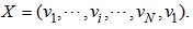 | (1) |
Each element vi is the i-th visiting city in a tour X, and N is the number of cities given in an instance. The total cost E(X) of X is shown as follow,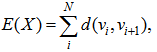 | (2) |
where d(vi,vi+1) is the cost of the edge e(vi,vi+1) between the vi and the vi+1 (i=1,…,N, vN+1=v1). The optimal tour X* is shown as follow,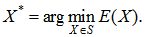 | (3) |
In Euclidean plane, the edge costs are defined as follow, 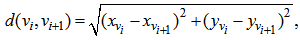 | (4) |
where xvi and yvi are the coordinates of a city vi.
2.2. Necessary Conditions for Optimality
Two necessary conditions that a tour is optimal in the Euclidean plane TSPs were proved; Flood[14] had proven that the optimal tour does not intersect itself, and Gonzales[15] had proven that the visiting order of the cities on convex hull in the optimal tour is the same as the order in which these cities appear on convex hull. Figure 1 shows the case of the instance berlin52 as an example for the second necessary condition for optimality.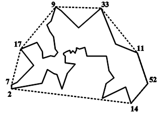 | Figure 1. An example for the second necessary condition. The numbers in this figure are the city labels on convex hull. The order which the cities are visited on the convex hull (broken line) in the optimal tour (solid line) is 2-14-52-11-33-9-17-7-2, and the order which the cities appear in the convex hull is also 2-14-52-11-33-9-17-7-2. Both orders are equal to each other |
2.3. Description of Shortest Hamiltonian Path Problem
A SHPP is to search a minimum cost path between the starting city vs and the terminating city vt visiting for each city v in the given city set V exactly once, and this constraint for the paths is expressed as S’. A SHPP can be solved as a standard TSP with the special edge cost between the vs and the vt[2]. A solution path Pvs,vt in S’ from the vs to the vt is expressed as follow, | (5) |
3. Theory of Proposed Framework
3.1. Alternative Description of TSP
Because the second necessary condition leads the optimal visiting order of the cities on convex hull, the optimal tour can be divided into some paths at the cities on convex hull with optimality. Such a city on convex hull C is called a terminal t. When the number of terminals is m, the number of paths is also m. The optimal tour X* can be replaced with the ordered terminals tj in C (j=1,…,m) as follow,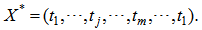 | (6) |
Hence, to obtain a tour we must decide all paths from tj to tj+1 (j=1,…,m, tm+1=t1). Then, at first, we should classify the cities v not in C into m subsets Vj (j=1,…,m) which construct sub problems as SHPPs through this classification problem as a sub problem. A subset Vj includes the terminals tj and tj+1. Secondly, we should solve each SHPP as sub problems to obtain the required paths Ptj,tj+1 from the starting city tj to the terminating city tj+1 in Vtj (j=1,…,m, jm+1=j1). The Vtj and Ptj,tj+1 are shown as follows, | (7) |
 | (8) |
where * is a meta character as a wild card to be replaced with classified cities. That is, a TSP in Euclidean plane can be replaced with a classification problem and m SHPPs. The equation (2) can be represented as follow,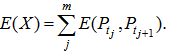 | (9) |
Then, a relation holds as follow,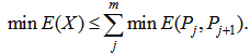 | (10) |
The equal sign holds when the classifications of the cities not on convex hull are optimal.
3.2. Replaced SHPPs with Special Conditions
The SHPPs which are converted from the TSPs have the two special conditions; (1) the starting city vs and the terminating city vt are neighbouring on convex hull C, and (2) the cities are distributed only in one side of the straight line connecting the vs and the vt. And it is clear that the terminals tj in the optimal path are also visited with the appearing order on the convex hull C. That is, the necessary conditions for optimality can be applied to the SHPPs in the same way for the TSPs. Furthermore, a SHPP also can be replaced with a classification problem and m SHPPs. Figure 2 shows the optimal path and the convex hull of a SHPP as a sub problem of the instance berlin52 in TSPLIB. This figure indicates that the second necessary condition is also kept in the SHPPs. | Figure 2. A SHPP as a sub problem of berlin52 in TSPLIB. Solid lines are the optimal path from the starting city 2 to the terminating city 14 in this sub problem, and broken lines are the convex hull of this city set |
As stated above, the SHPPs on our framework have the special condition in contrast with the standard SHPPs. The starting city vs and the terminating city vt are inevitably vs=t1 and vt=tm with the m terminals on the convex hull C. According to this condition, the SHPPs seem to be easier than the original TSPs.
3.3. Our Framework for the TSPs in Euclidean Plane
As shown in Figure 3, while repeating the replacements for each SHPP until the sub problems include only two cities, after all, the TSPs in Euclidean plane can be replaced only with the classification problems. 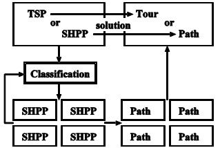 | Figure 3. The proposed framework for the TSPs in Euclidean plane |
Thus, the substance in our framework is the classifier for the cities vi not in C, and the quality of solutions depends on the error in the classifications. Alternatively, depending on the number or the distribution of the cities in the SHPPs, we should directly solve the SHPPs without the replacement.For example, Figure 4 shows the optimal classifications of the TSPLIB instance berlin52 when the instance is replaced only with the classification problems. The variable d is the depth in tree structure described in the next section. After the calculation of convex hull, the cities not on convex hull are classified into some subsets as SHPPs. And the convex hulls for each subset are also calculated. Finally, a solution tour is constructed through the process.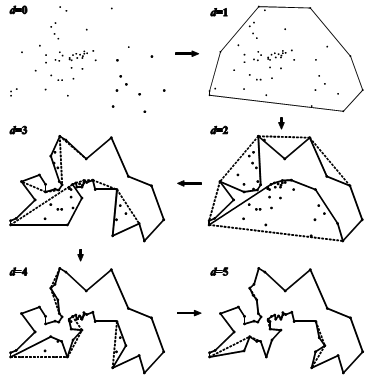 | Figure 4. The optimal classifications as the convex hulls of berlin52 in TSPLIB. The solid lines are the edges of convex hulls, and the broken lines are the edges replaced with some paths as solutions of SHPPs |
3.4. Tree Structure as a Tour
As our framework has the hierarchical process, the constructed tours through our procedure can be expressed in tree structure. In addition to, the tours, which have no intersect, are also expressed in tree structure by reverse calculation with our framework. For example, Figure 5 shows the tree structure of the optimal tour for the instance berlin52 in TSPLIB. The depth of the root node is d=0. This tree has maximal depth d=5 and all of the internal nodes as SHPPs corresponds the convex hulls in Figure 4 for each depth. In the tree structures, a tour is constructed by the leaf nodes with following in depth-first search.
4. Specifications for Our Framework
4.1. Implementation for Construction Methods
For the usage as construction methods, our framework needs only the setting of the classifier which the cities not on convex hull are classified into sub sets. We implement a pseudo code for construction methods on our framework in Figure 6 and describe the variables and the explanations of the pseudo code in this following.• N: the number of the cities in an instance.• V[]: the array for the city set, each element includes members x, y, label and key.• V[i].x: the coordinate x of a city V[i].• V[i].y: the coordinate y of a city V[i].• V[i].label: the label of a city V[i].• V[i].key: be used for the classification in sorting.• C[]: the array for the sub problems, each elements include members tail, head, size, depth, and parent.• C[i].tail: the starting index in V[].• C[i].head: the terminating index in V[].• C[i].size: the number of cities for each sub problem.• C[i].depth: the depth in tree structure.• C[i].parent: the parent problem for each sub problem. • num: the number of the sub problems.• start: the label of the starting city.• m: the number of the terminals on convex hull.• a: the number of generated sub problems.• p and q: the temporal variables for the range in V[].• i, j and k: the iterators for loops.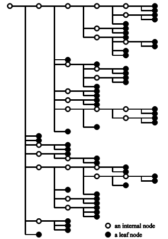 | Figure 5. The tree structure of the optimal tour of berlin52 in TSPLIB. Open circles are internal nodes in tree structuZre. The root node in the left side means a TSP and the other open circles mean SHPPs. Solid circles are leaf nodes that mean SHPPs which have only two cities. The leaf nodes are equal to the edges constructing a tour |
0. Lines 0-9: initialize the valuables, where the first problem C[1] is used for the original TSP.1. Lines 11-15: read the information of a problem C[i].2. Line 16: check the number of cities of C[i]. If the number is two, do not need calculate for the sub problem C[i].3. Line 17: call the function for calculating the convex hull of the C[i]. This function returns the ordered terminates tj (j=1,…,m) in appearing on convex hull in V[p..p+m-1]. We have implemented the function with Graham scan[16] which is suited to obtain the appearing order of the cities on convex hull.4. Line 18: adjust the order of the terminals so that the starting city is at V[p] and the terminating city is at V[p+m-1]. With the variable start which records the label of the starting city, we can obtain the correct order of the terminals.5. Lines 19-22: regulate a; the a is equal to m in the depth d=0, or equal to (m-1) in the depth greater than zero, because these sub problem do not use the path connected directly from vs to vt in the replaced SHPPs.6. Lines 23-25: terminals tj are labelled with j.7. Lines 26-28: the cities v not in C are classify into a subsets by labelling with the return number of the function for classification. The return number is the label of the generated subsets for the sub problems.8. Line 29: the cities V[p..q] are sorted with their key in ascending order. After this sorting, the cities are gathered for each sub problem.9. Lines 30-31: update the information of the generated sub problems C[num+1..num+a] by reading the V[p..q].key, where tail, head, size, depth and parent are calculated.10. Line 32: update the num incremented by a.11. Line 33: increment the iterator i.12. Lines 16-34: this procedure is looping while the iterator i is less than and equal to num.In this following, we describe the time and space complexity of the procedures working on our framework. At first, we define variables; Vi is a city set which has ni cities, mi is the number of the cities on convex hull Ci, and g(ni) is the computational cost in classification, where i is the iterator in the procedure. Then, we estimate the calculation cost for a loop in the next items,1. Read the problem information: w1.2. Check the number of cities: w2.3. Calculate the convex hull: w3ni log ni.4. Adjust the order of the terminals: w4mi.5. Label the terminals: w5mi6. Classify the cities not on convex hull: w6g(ni)7. Sort the cities: w7nilog ni.8. Update the cluster information: w8mi.Hence, the calculation cost f(ni) for the i-th loop is expressed as follow,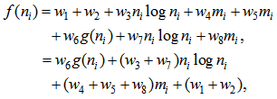 | (11) |
where wi is the suitable coefficients in computation for each procedure. If the cost g(ni) is equal to or less than nilog ni, the f(ni) is expressed with a coefficient w as follow, | (12) |
Otherwise, if the cost g(ni) is greater than nilog ni, the f(ni) is represented as follow, | (13) |
Then, by summation of (12) or (13) for all i, all of the calculation costs f(N) is represented as follow, | (14) |
 | Figure 6. A pseudo code for constructing methods on our framework |
where H is the total number of the clusters which excludes the two cities SHPPs as leaf nodes in tree structure because these problems do not need to be computed. The relation between H and all of the clusters M is shown as follow, | (15) |
To estimate the range of H, with the tree structure for TSP tours in our framework, we consider the influence when the sub sets, which the cities not on convex hull are classified into, are changed. These changes could be substituted for the moving of leaf nodes in the tree structure.At first, it is clear that each internal node inevitably has two or more child nodes except the root node which inevitably has three or more child nodes, because a TSP must have at least three cities for constructing a tour and also a SHPP must have at least two cities for constructing a path.In Figure 7, the movement of a leaf node u from the state (a) to the state (a)’ leads taking an increase of internal node at w with the shift of a leaf node from the place w to the place w’, while the movement of a leaf node v leads taking an decrease of internal node with the shift of the leaf node from the place v to the place v’. 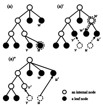 | Figure 7. The numerical changes of internal nodes |
If the internal node at the v’ has over three children, the movement of a leaf node take only an increase of internal node without a decrease. From the state (a) to the state (a)’’, the movement of the internal node u take only a decrease of internal node.Consequently, When the root node has all of the leaf nodes, the number of internal nodes is minimum as H=1, and when the root node has three child nodes and all of the internal nodes has two child nodes, which a child node is an internal node and the other is a leaf node, the number of internal nodes is maximum as H=N-2. Therefore, the range of H is shown as follow, | (16) |
And the calculation cost f(N) is represented with big O notation as follow,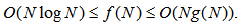 | (17) |
In addition, since the space needs O(N) without the procedure in classification, the space complexity is O(N) when the classification system requires the space which equal to or less than O(N).If the calculation costs for each classifications follow the equation (12), the time complexity is O(Nlog2N) and the space complexity is O(N). These orders appear when the optimal classifications as learning data in machine learning are generated with the optimal tour[12].
4.2. For Improvement Methods
After the running through our procedure, the solution tour could be improving with reclassifications of cities. We describe this idea with Figure 8 in this following.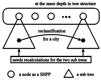 | Figure 8. An image for improvement procedure on our framework |
If a city or some cities are reclassified from a subset to another subset, the recalculations are needed for the two sub trees which are associated with this movement. The root nodes of these sub trees having the same parent at the same depth in tree structure. The tour improvement should be performed in such way while comparing the tour costs.Since the improving process is the recalculations for some sub trees, our framework could be applied to the methods which have the procedure depends on tree structure such as Genetic Programming (GP)[17],[18]. Insofar as we know, however, there is any method with GP for the TSPs though the many constraints will be required. If we achieve the construction of an effective method with GP, new intelligence may be given for the TSP.
4.3. For Parallel Computing
Because each sub problem independents of the other sub problems in the same level of tree structure, for the candidate patterns of classifications or for each sub problem, we could apply parallel computing to our framework easily though the implementation needs the experience in those technique.
5. Results and Discussion
5.1. As a Construction Method with a Simple Classifier
When we apply the simple function to the classifier, our framework will operate similar to classical methods. For example, we consider that the following equation is applied to the classifier,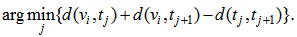 | (18) |
This equation means the increasing cost replacing the edge e(tj, tj+1) with the two edges e(vi, tj) and e(vi, tj+1) which incident to the city vi not in C. In this case, the time complexity is O(Nlog2N) and the space complexity is O(N). The solutions with this classifier have 20 - 30 percent error in the EUC_2D instances of TSPLIB.
5.2. Generated SHPP Benchmarks
The learning data for machine learning can be generated with the optimal tours of which the instances had been solved completely such as the EUC_2D TSPLIB instances. Accordingly, the optimal classifications can be regarded as the benchmark instances of the SHPPs. In Figure 9, we show that how many instances we can generate as the SHPP benchmarks with the TSPLIB instances. The x-axis indicates the number of cities as SHPP instances in log scale, and the y-axis indicates the frequency of the SHPP problems in log scale. There are many instances of the SHPPs enough to study the classifier on our framework.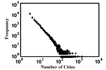 | Figure 9. The distribution of the number which the TSPLIB instances can generate the SHPP instances |
However, there is only slight knowledge and experience in constructing of machine learning system for the classifications. Thus, we should begin the training with small size SHPPs through trial and error. At the beginning, as the first goal in our study, we aim that a classifier trained in machine learning achieves the optimal classification in small size instances of the SHPPs.
5.3. About the Optimal Classification
Although we can construct a classifier in machine learning systems only with the geometric information such as the coordinates of cities, however, through generating the learning data for the TSPLIB instances with the optimal tours, the optimal classifications provide us the knowledge that the convex hulls generated as the optimal classifications are frequently overlapping each other in geometry. These overlaps appear in the instances which have over 100 cities. Figure 10 shows an example of the overlapping in optimal classification for the instance d15112 of TSPLIB. These convex hulls are at the depth d=1 in tree structure. There are 21 internal nodes as convex hulls and 2 leaf nodes as edges. This matter exhibits that only the simple geometric information such as the equation (18) cannot generate the optimal classifications, and that the topological information such as a minimum spanning tree will be essential to realize the optimal classifications. Consequently, for the classifiers in machine learning, we must use quantity of many various features not only the geometric information but also the topological information through trial and error.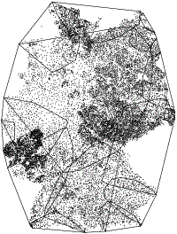 | Figure 10. The overlapping of the convex hulls at the depth d=1 in the optimal classifications for the TSPLIB instance d15112 |
6. Conclusions
We have proposed the theoretical framework to solve the TSPs in Euclidean plane as a classification problem and some SHPPs. The necessary conditions or optimality can replace the TSPs with a classification problem and some SHPPs. The replaced SHPPs as sub problems have the two special conditions; (1) the starting city and the terminating city are neighbouring on convex hull and (2) the cities are distributed in one side of the straight line connecting the starting city and the terminating city. The SHPPs also can be replaced with a classification problem and some SHPPs in the same way for the TSPs, which leads that the TSPs are replaced with only classification problems. If the classifications are optimal, the solution is also optimal. The performance of the proposed framework depends on the applied classifier in quality and complexity. We conjecture easily that the classification problems are very difficult to be solved with the simple classifiers, because the optimal classifications are overlapping in the instances which have over 100 cities.Therefore, the main theme of the proposed framework is the study of the classifiers. We showed the specifications as several approaches with the framework for the TSPs. And with the TSPLIB instance, we can generate many SHPP instances of which the optimal solutions can be obtained. Through the study of the classifiers for the SHPPs from small size instances to large size instances, we expect the achievement to acquire the effective intelligence for the TSPs with our framework in future work.
References
| [1] | E. L. Lawler, J. K. Lenstra, A. H. G. Rinnooy Kan and D. B. Shmoys, Ed, "THE TRAVELING SALESMAN PROBLEM", John Wiley & Sons, 1985. |
| [2] | Gerhard Reinelt, "The Traveling Salesman: Computational Solutions for TSP Applications", Berlin Heidelberg, Springer-Varlag, 1994. |
| [3] | G. Gutin and A. P. Punnen, Ed, "The Traveling Salesman Problem and Its Variations", Kluwer Academic Publishers, 2002. |
| [4] | Concorde, Online Available:http://www.math.uwaterloo.ca/tsp/concorde/index.html. |
| [5] | TSPLIB95, Online Available:http://comopt.ifi.uni-heidelberg.de/software/TSPLIB95/index.html. |
| [6] | K. Helsgaun, "An Effective Implementation of the Lin-Kernighan Traveling Salesman Heuristic," European Journal of Operational Research 126(1), pp.106-130, 2000. |
| [7] | LKH2, Online Available:http://www.akira.ruc.dk/~keld/research/LKH/index.html. |
| [8] | DIMACS TSP Challenge, Online Available:http://dimacs.rutgers.edu/Challenges/TSP/ |
| [9] | S. Lin and B. W. Kernighan, "An effective heuristic algorithm for the traveling-salesman problem," Operations Research 21, pp.498-516, 1973. |
| [10] | D. Applegate, R. Bixby, V. Chvatal, W. Cook, D. Espinoza, M. Goycoolea and K. Helsgaun, "Certification of an optimal TSP tour through 85900 cities," Operations Research Letters 37, pp.11-15, 2009. |
| [11] | S. Eilon, C. D. T. Watson-Gandy and N. Christofides, "Distribution management: Mathematical modelling and practical analysis," London: Griffin, pp.113-150, 1971. |
| [12] | O. Mersmann, B. Bischi, J. Bossek, H. Trautmann, M. Wagner and F. Neumann, "Local Search and the Traveling Salesman Problem: A Feature-Based Characterization of Problem Hardness," Learning and Intelligent Optimization, pp.115-129, 2012. |
| [13] | A. Kawashima and Y. Sugai, "A Generator of Learning Data for the TSPs Based on the Visiting Order of the Cities on Convex Hull," IEEE Multi-Conference on System and Control, FrC04-1, pp.2302-2307, 2010. |
| [14] | M. Flood, "The traveling salesman problem," Operations Research 4, pp.61-75, 1956. |
| [15] | R. H. Gonzales, "Solution to the traveling salesman problem by dynamic programming on the hypercube," Technical Reports No. 18, Operations Research Center, M.I.T., 1962. |
| [16] | R. L. Graham, "An Efficient Algorithm for Determining the Convex Hull of a Finite Planar Set," Information Processing Letters, vol.1, pp.132-133, 1972. |
| [17] | John R. Koza, "Hierarchical genetic algorithms operating on populations of computer programs," Proceedings of the Eleventh International Joint Conference on Artificial Intelligence IJCAI-89, pp.768-774, 1989. |
| [18] | J. R. Koza, "Genetic Programming: A Paradigm for Genetically Breeding Populations of Computer Programs to Solve Problems," Stanford University Computer Science Department technical report, STAN-CS-90-1314, June 1990. |
 Abstract
 Reference
 Full-Text PDF
 Full-text HTML