1. Introduction

Fuzzy time series procedures do not require the assumptions such as the large sample and that the model is true. Recent studies are about fuzzy time series procedures since they do not require the strict assumptions and generally provide remarkable forecasting performances.

The fuzzy set was firstly introduced by Zadeh[1] and this concept has found many application areas since then. Fuzzy time series were introduced firstly in the studies of[2, 3, 4]. These proposed fuzzy time series techniques in literature generally consist of the three stages; these are fuzzification, determining of fuzzy relations and defuzzification.In the literature, the decomposition of universe of discourse was mostly used in the fuzzification stage and intervals of it was determined arbitrarily the studies of[2, 3, 4, 5,6]. In addition, Huarng[7] has put forward the importance of the interval length on the forecasting performance and proposed two new techniques based on the mean and the distribution in order to find intervals. Egrioglu et al.[8, 9] have suggested forming the problem of finding intervals as an optimization problem.

Chen and Chung[10] and Lee et al.[11] used genetic algorithm to find the interval lengths, and also Fu et al.[12], Huang et al.[13], Kuo et al.[14, 15], Davari et al.[16], Park et al.[17] and Hsu et al.[18] used the particle swarm optimization. Besides these studies, Cheng et al.[19] and Li et al.[20] used fuzzy C-means clustering method in their studies and also Egrioglu et al.[21] used Gustafson-Kessel fuzzy clustering method in this stage.

In the stageof determining of fuzzy relations, while Song and Chissom[2, 3, 4] used matrix operations, Chen[5] and some others were used the fuzzy logic relations group table and also artificial neural networks were used in the studies of[7, 22, 23, 24, 25, 26] for determining the fuzzy relations. The other studies in this stage were proposed in the studies of[23, 27, 28, 29].

In defuzzification stage, studies in the literature mostly used the centroid method. Chen[5], Huarng[7]. Cheng et al.[30], Aladag et al.[28] preferred to use adaptive expectation method in the defuzzification process.

The determining of the fuzzy relations is very important for the model structure. Besides, the forecasting performance may be improved if the fuzzy relations defined well.

From this point of view, we used Differential Evaluation Algorithm (DEA) in fuzzification stage to avoid subjective decisions and also we aimed to obtain more realistic forecasts by using fuzzy relations recurrence numbers. Because, using recurrence numbers of fuzzy relations is important as well as fuzzy relations occur or not.

In this study, a fuzzy time series approach that uses DEA in fuzzification stage and takes into account the recurrence numbers of fuzzy relations was proposed and also the proposed method was supported by the applications and it is superior forecasting performance was shown.

The rest part of the paper can be outlined as below: The fundamental definitions of fuzzy time series has been given in Section 2. Short information about DEAhas been given in Section 3. In Section 4, the proposed method has been introduced. In Section 5, the results from the application of the proposed method to three real life data sets have presented. In section 6, discussionshave been presented and finally in section 7, conclusions havebeen presented.

2. Fuzzy Time Series

The definition of fuzzy time series was firstly introduced by Song and Chissom[2, 3, 4]. In contrast to conventional time series methods, various theoretical assumptions do not need to be checked in fuzzy time series approaches. The most important advantage of the fuzzy time series approaches is to be able to work with a very small set of data.

Let U be the universe of discourse,where . A fuzzy set of U can be defined as,

(1)

Where is the membership function of the fuzzy set and .

In addition to, denotes is a generic element of fuzzy set is the degree of belongingness of to.

Definition 1 Let , a subset of real numbers, be the universe of discourse by which fuzzy sets are defined. If is a collection of then is called a fuzzy time series defined on Y(t).

Definition 2 Fuzzy time series relationships assume that is caused only by then the relationship can be expressed as: , which is the fuzzy relationship between andwhere * represents as an operator. To sum up, let and . The fuzzy logical relationship between and can be denoted as where (current state) refers to the left-hand side and (next state) refers to the right-hand side of the fuzzy logical relationship. Furthermore, these fuzzy logical relationships can be grouped to establish different fuzzy relationship.

3. Differential Evaluation Algorithm

DEA was proposed by Price and Storn[31]. DEA is a heuristic algorithm based on the population. It has some operators such as mutation and crossover operations. These operators are used to create new generations. At the end of the process, candidate solutions are found by using some mathematical operations and these solutions are compared with the current solutions in the population. The best solution is transferred to the new generation according to the evaluation function and the best chromosome is taken as the optimal solution. DEA and its operators discussed in more detail in the section of proposed method and also those who want more information can look the study of Price and Storn[31].

4. Proposed Method

As it is well known that all stages of the fuzzy time series approaches influences very much intensively on the forecasting performance of the applied model and researchers have used different techniques to make a contribution to each stages. In recent years, artificial intelligence algorithms have been used in fuzzification stage by the researchers and also the researchers have generally preferred to use the centroid method in the last stage so far and also the stage of determining of the fuzzy relations is very important as well as the other stages of fuzzy time series approaches. Besides, the forecasting performance may be improved if the fuzzy relations defined well. From this point of view; we have noticed that none of them have considered how many times a fuzzy relation has occurred.

To overcome this problem, the weights can be given for each fuzzy relation according to their recurrences. Then, these weights can be used in the defuzzification stage. Because using recurrence numbers of fuzzy relations is important as well as fuzzy relations occur or not and the forecasting performance may be improved with the help of using these recurrence numbers

In this study, a fuzzy time series method that uses DEA in fuzzification stage and takes into consideration of recurrence numbers of fuzzy relations in defuzzification stage to obtain more realistic forecasts has been proposed.

The main advantages of proposed method are as follows:

• The interval lengths are determined by avoiding subjective decisions because of using DEA.

• A more flexible solution process is provided by obtaining fix interval length instead of constant length interval.

• The most basic element in the structure of the model is fuzzy relations. To obtain forecasts as well as the fuzzy relations, using their recurrence numbers cause to obtain more realistic forecasts.

• The search space has been differentiated by using DEA and new generations are obtained.

Briefly, we can summarize our proposed method as below.

Algorithm.

Step 1 and are the minimum and maximum values of time series, respectively and the universe of discourse is defined in Equation 2.

(2)

andare the numbers determined arbitrarily.

If genes are shown with a chromosome structure of DEA can be shown as follows.

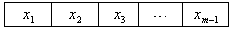Figure 1. A chromosome structure of DEA

According to the values of these genes, the parts of universe of discourse, i.e., sub-intervals are shown as follows:

(3)

Step 2 The generation of initial population.

is to show the n. gene of k. chromosome of j. generation

(4)

The genes produced by chromosomes are sorted by ascending order.

Step 3 For each chromosome in the population, the root of the mean squared error (RMSE) selected as the evaluation function is calculated by applying the steps from 3.1 to 3.5.

Step 3.1 m intervals based on the values of genes in chromosomes are used to form fuzzy sets as below.

(5)

here, is the membership degrees and it is shown in equation 6.

(6)

The observations of crisp time series are converted to the fuzzy sets in which the interval in which the corresponding observation is included, has got the highest degrees of membership value.

Step 3.2 Obtainthe FLRs and FLRG tables.

For example, when we observe the relation such as and for any time t this fuzzy logic relation is represented by . In the whole series if we get the relation and for any time t then we express the fuzzy logic relation as . Also we save the number of how many times the fuzzy logic relation such as is occurred, into the weights .

Step 3.3 Obtain the fuzzy forecasts.

The fuzzy forecasts are obtained with respect to the fuzzy logic relation table. If and there is a relation such as in the fuzzy logic relation table then the fuzzy forecast will be. If and there is a relation such as in the fuzzy logic relation table then the fuzzy forecast will be If and in the fuzzy logic relation table then the fuzzy forecast will be.

Step 3.4 Defuzzify the fuzzy forecasts.

The weights obtained from the fuzzy logic relation table are used in the defuzzification stage.

For example; If and there exists the relation in the table then the defuzzified forecast will be which is the midpoint of which is the subinterval of the fuzzy set with the largest membership degree. That is, we don’t regard how many times that relation is repeated in the table.

If and there exists the relation and is the number of how many times the relation is repeated in the whole time series and is the number of how many times the relation is repeated then the defuzzified forecast is calculated as below.

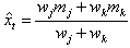(7)

If and there exists the relation in the fuzzy logic relation table then the defuzzified forecast will be which is the midpoint of the subinterval which is the fuzzy set with the largest membership degree.

Step 3.5 Let be the original time series and be its defuzzified forecasts with the nobservations. RMSE is calculated by the equation 8.

(8)

Step 4 utation and Crossover operations.

Mutation and Crossover operations are applied to for each chromosome(Chr) in the initial population, respectively.

Step 4.1 The application of Mutation operation

For applying mutation operation in DEA, firstly we choose four chromosomes. The first one of these four chromosomes is called as current chromosome and the remaining three chromosomes are selected randomly except current chromosome.

The first two of these selected three chromosomes are subtracted each other and it is called as the difference vector.Then, difference vector is multiply by F and a new chromosome is obtained (In general the parameter F gets values between 0 and 2. We take this F value as 0.8 which is general value in the literature in this study). This new chromosome is called as the weighted difference vector. The weighted difference vector is summed with the third chromosome and mutation is completed. This new created chromosome is called as the total vector.

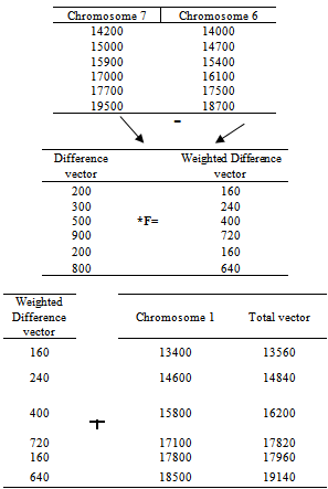Figure 2. An example of mutation operation

Table 1. An example of a random population

Thus, the chromosome to be used in the crossover operation is created with the help of mutation operation.

To better understand mutation operation, let’s look at the Figure 2 and take a population with 7 chromosomes and the universe of discourse is as given in Table 1. and assume that the Chromosome 2 is the chromosome to be mutated and Chromosome 6, Chromosome 7, Chromosome 1 are the chromosomes selected randomly except Chromosome 2.

Step 4.2 The application of Crossover.

To apply Crossover operation, the total vector obtained from at the end of the mutation operation is compared with current chromosome and nominee chromosome is obtained.

While nominee chromosome is obtained, each gene of total vector and current chromosome is evaluated one by one.

First at all, a crossover rate (cor) is determined. Then, a random number is generated between 0 and 1 with the help of uniform distribution.

If this random number is smaller than the crossover rate, the gene is taken from total vector. If it is not, the gene is taken from currentchromosome and nominee chromosome is generated and the fitness value of nominee chromosome is calculated.

Then, let’s determine the (cor) rate. For example let’s take it 0.10 than generate random numbers for each gene, respectively. (0.01, 0.08, 0.15, 0.20, 0.16) and obtain the nominee chromosome. An example of crossover has been given in Figure 3.

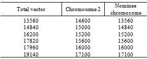Figure 3. An example of Crossover

Step 5 The comparison of fitness values

Nominee chromosome and current chromosome are compared in terms of fitness values. The chromosome which has the smaller RMSE value used as evaluation function is transferred to new generation. For example let’s assume that the RMSE value of Nominee chromosome is smaller than chromosome 2 then, nominee chromosome is transferred to the new generation like shown in Table 2.

Table 2. An example of creation of a new generation

All these operations are applied to each chromosome in initial population individually.

Step 6 Steps 3-5 are repeated as much as a predetermined number of iterations.

5. Application

In order to show the performance of the proposed method this is applied to three different time series data. The results are compared with the results from the methods which are already in fuzzy time series literature with regards to RMSE and Mean Absolute Percent Error (MAPE) criteria.

(9)

For each time series data DEA parameters are defined as follows.

• cn is experimented as from 10 to 100 with increment 10

• cor is experimented respectively 0.1 to 1 with increment 0.1

• m is experimented as from 5 to 20 with the increment 1.

• For all possible case, DEA is executed 100 times in MATLAB.

At the end of the process, we obtained 1600 different solutions. Then the parameters (m, cn, cor) with the smallest RMSE value were taken as the best solution among these solutions.

5.1. Enrollment Data

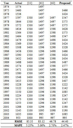
The performance of proposed method is evaluated separately for both test and training sets for enrollment data between the years 1971 and 1992. Firstly all data is used for training set like almost all studies in the literature and then the last three observations of enrollment data is taken as test set and it is compared with the other studies in the literature. It is clearly seen that our proposed method has superior forecasting performance.

As a first experiment, the proposed method is solved for training data. We conclude that the best result is obtained in the case where m=19, cn=80, cor=0.9. Table 3 presents the all results, which include forecasts and the RMSE and MAPEvalues, obtained from the proposed method and the other methods proposed in literature, comparatively. These results from both are belonging to the best case.

Additionally, a comparative presentation of enrollments’ forecasts in terms of RMSE values for some other methods is given Table 4.

As a second experiment, the proposed method is solved for test data. We conclude that the best result is obtained in the case where m=16, cn=60, cor=0.3. Table 5 presents the all results, which include RMSE values, obtained from the proposed method and the other methods proposed in literature, comparatively.

5.2. Taifex Data

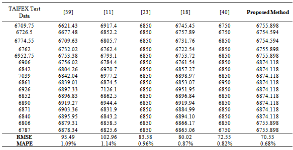
In the second case, the proposed method was applied to TAIFEX data whose observations are between 03.08.1998 and 30.09.1998. The last 16 observations are used for test set, respectively. We conclude that the best result is obtained in the case where m=12, cn=70, cor=0.9. Table 6 presents the all results, which include forecasts and the RMSE and MAPE values, obtained from the proposed method and the other methods proposed in literature, comparatively. These results from both are belonging to the best case.

Table 3. A comparative presentation of enrollments’ forecasts for training data

Table 4. A comparative of enrollments’ forecasts for training set in terms of RMSE

Table 5. The comparison of the results for test set data

Table 6. The comparison of the results for test data

5.3. Car Road Accident in Belgium Data

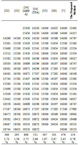
In the third case, the proposed method was implemented on the time series data of ‘killed in car road accident in Belgium’. We conclude that the best result is obtained in the case where m=20, cn=80, cor=0.2. Table 7 presents the all results, which include forecasts and the RMSE and MAPE values, obtained from the proposed method and the other methods proposed in literature, comparatively. These results from both are belonging to the best case.

As seen in Table 7, the method we propose gives the best result with respect to the forecasting performance.

6. Discussions

Using recurrence numbers of fuzzy relations is important as well as fuzzy relations occur or not.And also the forecasting performance may be improved with the help of using these recurrence numbers of fuzzy relations Besides, more reliable results may be obtained by giving weights as the number of repetitions of recurrent fuzzy relations. Besides, the contribution of fuzzy relations recurrent more is more than the fuzzy relations recurrent less. We also considered this contribution and gave more weights to the fuzzy relations recurrent more.

Table 7. A comparative presentation of killed forecasts and the actual observations by various methods

7. Conclusions

Fuzzy time series forecasting methods have attracted much attention in recent years. Different approaches have been proposed for the each stage of fuzzy time series approaches. The stage of determining of fuzzy relation is very important for fuzzy time series approachesbecause it affects defuzzification stage. Revealing the effects of fuzzy relations, properly may improve the forecasting performance. From this point of view, we used DEA in fuzzification stage to avoid subjective decisions and also we consider the recurrence numbers of the repeated relations in fuzzy logic relation table which is necessary in the defuzzification stage in this study. By using recurrence numbers of fuzzy relations the forecasting performance was improved. The proposed method was supported by the real data sets analysis and its superior forecasting performance was shown.

We expect that in future studies researchers can concentrate on a different optimization technique for finding the weights used in the defuzzification stage and may use different artificial intelligence techniques in fuzzification stage.