Afsoon Assa, Majid Vafaei Jahan
Department of Computer Engineering, Islamic Azad University, Mashhad Branch, Mashhad, Iran
Correspondence to: Majid Vafaei Jahan, Department of Computer Engineering, Islamic Azad University, Mashhad Branch, Mashhad, Iran.
| Email: |  |
Copyright © 2012 Scientific & Academic Publishing. All Rights Reserved.
Abstract
Recent advances in wireless sensor network's technology have developed using this technology in various fields. For the importance and intense application of these networks, many efforts and researchers have been done to confront challenges. In this paper, to conquer one of the most important challenges of these networks, that is the limitation in energy resources, an adaptive scheduling algorithm based in Potts model was applied. According to this model, for every element within a system, q different states are considered. Each element converts its state to a new state or remains in that state due to its current state and its adjacent neighbours and with the effect of environment. In this project, this model was used in wireless sensor networks such that each sensor node is considered as an element of sensor network system and three active, inactive and standby states are defined for that node, which it selects one of these three states according to its current state and neighbours and environment affect and adapts its activity on the environment in a way that the least energy to be consumed. By comparing this algorithm and similar algorithm (with two states), it is observed that in identical conditions, Potts model with three states represent better results and more lifetimes for network.
Keywords:
Ising Model, Markov Random Field (MRF), Potts Model, Wireless Sensor Networks (Wsns)
Cite this paper:
Afsoon Assa, Majid Vafaei Jahan, "Adaptive Scheduling in Wireless Sensor Networks Based on Potts Model", American Journal of Intelligent Systems, Vol. 2 No. 7, 2012, pp. 157-162. doi: 10.5923/j.ajis.20120207.01.
1. Introduction
Wireless Sensor Networks (WSNs)[1] consist of the limited resources constrained devices, called sensor node, which communicate wirelessly to one another. These nodes are able to recognize changes of states occur in their impact domain and to report processed obtained data to respective centres. This property causes usage of this technology various applications. One of them are to track a target which is used in different applications in benign environments and also harsh ones. As mentioned previously, these networks were comprised of nodes with limited energy resources; therefore, one of the most important challenges of these networks is energy limitation and attempt to increase the operational lifetime of network. To use effectively of sensor networks, which have been different spins.requires resource-aware operation and takes care of a resource as much as possible; this is because sensor nodes are distributed only once, and resources of sensor nodes are hardly ever rechargeable. To decrease energy consumption of network, it is usually tried to reduce node's duty cycles, but in such applications of Sensor networks for event detection and tracking, it is impossible to use a fixed rule to decrease node's duty cycles because events of interest are often rare and unpredictable. So if operational cycles of Nodes are reduced, when nodes are not active, an event may occur, which its incorrect detection and tracking led to serious consequences and irreparable losses. Many researches were done due to wireless sensor Networks's challenge and energy saving of these Networks, particularly in application of target tracking and various algorithms has been designed. One of these algorithms is an algorithm of adaptive sensor activity scheduling (A-SAS) algorithm[2] in distributed sensor networks, where the sensor network is modeled as a Markov random field on a graph. The sleep and wake modes of a sensor node are modeled as spins with ferromagnetic neighborhood interactions in the Statistical Mechanics setting. According to this algorithm, node's activities are scheduled such that network nodes could be able to detect targets all the time and determine the target's path correctly. The main goal of this paper is to develop the algorithm such that besides detect objective correctly, nodes to be scheduled in a way that to consume the least energy. In the proposed algorithm, Potts model was used to develop the algorithm. The paper is organized in four sections, including the present one. In section 2, Ising model and Potts model will be introduced. The proposed algorithm will be studied in section 3. In section 4, after evaluating algorithm efficiency, the algorithm will be compared with Ising model with the same conditions, and in the last section, conclusions will be given.
2. Introducing to Ising and Potts Model
The Potts model studies long term behaviour of complex systems. The model is able to investigate how the internal element of the system reacts with each other based on certain characteristics that each element has. As these reactions take place macroscopic properties of the system will evolve. The Potts model has proven to be a very useful tool for simulating real systems. This model is used in the area of mathematical modelling so called statistical mechanics. In this model, the system is mapped to a graph such that graph nodes are the comprising elements of the system, and its edges are the connections among these elements. For many applications, it is expedient to presume that the graph has a regular structure, such as a lattice. On the vertices of these graphs, anything can be considered, like atom, human, liquids and cells and even sensor node. Potts model models how the nearest elements with different spins are related to other elements of the lattice[3]. This model is the extended of Ising model[4,5]. In Ising model, two states are considered for each vertex, but in Potts model, q different states can be considered for every vertex. Since the elements are assigned different spins and reacts with one another depending on their position on the lattice and their specific spins, there will be some measure of overall energy of the system. The function which measures the overall energy of a complex is the Hamiltonian[6]. 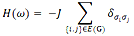 | (1) |
Where, J is the interaction energy between adjacent elements of the system, and σi is the spin value assigned to vertex i in the state ω, and a 1 is placed on edges between neighbors with like spins and a 0 on edges with elements which have been different spins.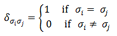
2.1. The Potts Model Partition Function
For a graph with n vertices which its vertex can have q different spins, there are qn states. In fact, Potts model studies these states. The Potts model probability function is the function which calculates the probability of finding the lattice in a particular state. This function depends on the Boltzmann distribution in statistical mechanics. Equation 2 shows above function with exponential distribution.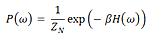 | (2) |
Where,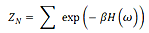 | (3) |
Equation (3) is called Partition function of this model. Therefore: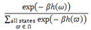 | (4) |
This equation computes the probability of finding a particular state ω in possible states set Ω, where,  , T represents the temperature of the system, and k = 1.38 × 10⁻²³ (joules/Kelvin) is the Boltzmann constant. However, computing the partition function is only tractable for small lattices and small values of q. In general, this function is NP-hard to compute. Mathematicians explore properties of the Potts model partition function in a variety of ways. One way is to interpret it as an evaluation of the Tutte polynomial[7]. Another is to approximate the function using a simulation technique such as the Metropolis Algorithm[8]. This calculation is not exact; however, it allows researchers to use the Potts model to investigate complex applications.
3. The Proposed Method
The idea of using Potts model in wireless sensor networks was expressed in an algorithm called A-SAS[2]. This algorithm is a distributed algorithm for wireless sensor networks to be able to detect and track rare and random events. However, in this algorithm, Ising model was used, that is for sensor node, just two active and inactive states were considered.The algorithm which is represented here is extended of A-SAS algorithm using Potts model. Therefore, instead of two states for nodes, three states are considered and the third state as standby is added. The sensor nodes are presumed to be equipped with relevant sensing transducers and data processing algorithms as needed for detection and tracking of events under consideration. Node's task is that until resources are available, they detect and track rare events. Problem assumptions: (1) the network only deployed once. (2) Sensor nodes are static. The neighbours are fixed and predetermined. (3) Sensor node connected to its nearest neighbours through a short single-hop wireless communication.Sensor network is considered as a weighted graph. If G ≜ (S, E, W) is supposed a weighted graph where S = {s1, s2, ... sN} and N ∈ℕ is the set of all nodes of the sensor network and E is the set of all edges of graph G which each edge specifies the distance between two nodes of S that are connected together with single-hop and is determined by an edge (si, sj) ∈ E. Function W expresses the weight of the graph's edge and has the value W((si, sj)) = wij. The strength of interaction this function is dictated by factors such as physical distance between the sensor nodes.To describe the problem, some definitions have to be stated: (1) Markov Random Field: suppose ∂ ≜ {∂i} si ∈ S be the neighbour set for a node si. Then, with respect to ∂, a random field is called a Markov Random Field (MRF) if and only if hold the Markov properties (I.e. P(wi ∣ K∂i) = P(wi∣KS\{i}))[9]. where, K S\{i} and K∂i are configurations specified for node set S\{i} and ∂i, respectively; P is the probability of random field F. This condition of Markov property ensures that the probability of a node being in a state depends only on its neighbours. (2) a set of nodes, c, which is a subset of S or equal to S (c ⊆ S) is called a clique, If a graph which has been induced on c by G is complete (that is each two nodes in G have mutual neighbourhood with each other)[10]. (3) The Hamiltonian or energy function for a configuration K is defined as: | (5) |
3.1. Formulating Potts Model for a Sensor Network
In this section, Potts model of a sensor network, which was introduced as a Markov random field on graph G, is formulated. The rationale is that the behavior of a sensor node would depend strongly on its nearest neighbors and would be relatively unaffected by the decisions of a distant node. Sensor nodes introduce as binary random variables and the potential of each clique is determined. This potential is used for modelling the behaviour of nodes. The objective here is to achieve the desired activity of the sensor network with a distributed probabilistic approach as explained below. The State (or label) set is selected as Ω = {active, inactive, standby}, to be a discrete set. Random field F is defined as:Fi : Ω → {-1, +1, 0.1}, ∀i = 1, 2,…, NAnd the clique potentials are defined as: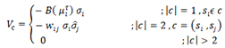 | (6) |
Where |c| is the basis for determining the potential;  is the time τ-dependent value of the node si depend on time τ;
  is as a defined function
  ; and
; and  is the expected value of σ j. It should be noted that Vc (σi , σj) ≠ Vc (σj , σi). In the Potts-model,
  corresponds to the external magnetic field and wij to the coupling constant[11] is assumed to be strictly positive. Cliques of size more than two would require to investigate of neighbours of neighbours, which become cumbersome for a large |c|. Therefore, from the implementation vision, cliques with size greater than 2 are not raised in the formulation and the potential value will be considered as zero. The Hamilton that shows the energy of the K configuration is now written in terms of the potentials Vc as:
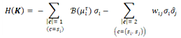 | (7) |
According to equation (4), for supposed configuration K, conditional probability P(wi ∣ K S\{i}) is expressed as:  | (8) |
Where, Ci is the set of all cliques containing node si; and K’ is a configuration of K in which node si is labelled with w’i. Assume that ∆H (σi) be node si energy changes with its state change from one state into another. For node si, the probability of activeness via equation (8) is stated as: | (9) |
Obtained results show that the probability of being active  , is a function of current state of node si and expecting behaviour of its neighbours. Without of magnetic-field
  indicating the external effect in the sense of a function of
  , the node probabilities are only dependent on its neighbours. Sensor network system would have a fixed point at P* = 0.5. The fixed point of the system determines when there is no event in the sensor field, system's operations properties to be usual and natural (μi =0 ∀i). Thus, for a sensor network application, the ability to choose P* would be desirable. For a given 0< P*<1, this is accomplished as follows. Let clique potentials be defined as:
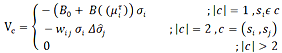 | (10) |
Where, | (11) |
And  be the change in expecting spin of the neighbor. For considered P*,
  Therefore,
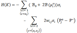 | (12) |
And according equation (11) and (12), it is obtained that: | (13) |
Due to these equations, for the moment that node si senses an event around itself, According to the state of node si and its neighbours, delta calculated, and it is placed in equation (9) to obtain the probability of being active. The formulation that presented here essentially follows a hybrid model[12] where the clique potentials and the probabilities are functions of two variables, a discrete variable (μi) and a continuous variable . To adapt to the dynamic operational environment, sensor nodes recursively calculate their probabilities based on their interactions of neighbours and most recently sensed data.
3.2. Experimental Results
To implement this algorithm, OPNET simulating software was used[13]. Sensor network is simulated with two-dimensional of sensor nodes (like[14] or[15]). Sensor network was formed with nodes 35 (7*5) that exposure in the uniform network. Each node has four neighbours nearest orthogonal, with inter-node distance between the neighbors being set to 2.5 units. Note that with nearest orthogonal neighbors, cliques of order 3 or more are not present. The measurable value μi is taken to balanced (normalized) the signal intensity that detected by the sensor node si. Figure 1 illustrates this network. Each node of it is considered as a Markov random field with three states. Figure 2 represents a node of sensor network.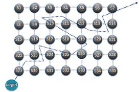 | Figure 1. wireless sensor network |
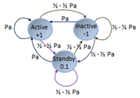 | Figure 2. a node of graph with three active, inactive and standby states |
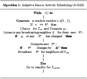
For each sensor node can be considered four different Modes: (1) active (Sensing and snaffing for messages from neighbors); (2) inactive (neither sensing nor receiving); (3) standby (neither sensing nor receiving, in fact this mode is a status of inactive mode that, sensors work in low power but wake up with a speed about 5 to 10 microseconds[16]) and; (4) transition (sending new pa to neighbours).Each pair of sensor nodes can be Exchange the information only if any two nodes are in active state and communication mode. Activity of a sensor network is scheduling with a random update of node states, which is shown in Algorithm 1. In a discrete scheduling, node si computes based on current
  in each time step, and identified neighbour's probabilities and broadcasts them to neighbours (note that in each broadcasting, sending packet is sent to those neighbor nodes, which are in distance w from node si). Nodes broadcast new
  only when it changes with by
  . This is done so that insignificant changes in
  are not broadcasted. Then, a sensor node assigns a state active, inactive or stand by in this time step with a probability of
  for active state and
  for inactive and standby states to itself. The stochastic local decision is to adapt to environment. To change the state of nodes, each node acts as following; if
  is greater than
 , node si assigns active state to itself and otherwise, since the probabilities of inactive and standby states are the same, it generates a random number. If generated number is greater than P*, node goes into standby state, otherwise converts into inactive one.
Algorithm 1. A-SAS with Potts model
 |
| |
|
Suppose that the network of figure 1 was embedded in a border region to track enemy infiltration, and it wants to pass a path which is determined on the scheme. Sensor nodes detect considered target along the path and declare obtained results from their detection to data sink. In the proposed algorithm, neighborhood interaction enables a sensor node to schedule its activity for an event occurring in its vicinity. To show the effects of neighborhood interaction, the event is simulated to be detected by only one sensor node. With respect to figure 1, in initial moments, the first the only node which detects the target is s29, this condition will be shown in pa computation by setting μ29=1 for s29 and μi=0 for all nodes si that i≠29. Other parameters P*,  w and B1 are set 0.3, 0.2, 2.5 and 10, respectively. In this algorithm for change on the activity probability to broadcast pa to all neighbors, δpa considered to be equal to 0.02. In algorithm 1,
  ,
, 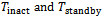 which are time durations of active, inactive and standby states, respectively, are taken values 1, 2 and 1 seconds, here. Also, the ratio of energy consumption in each state and node state conversion into active one is defined as:EInactive < Estandby < Estandby_to_active < EInactive_to_active < Eactive
4. Evaluating algorithm efficiency
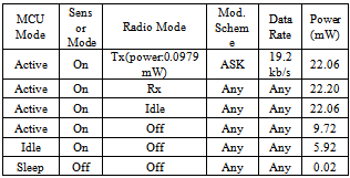
To evaluate the above algorithm efficiency, both algorithms were simulated and the results were recorded. Table 2 shows lattice lifetime (in terms of sec) in Potts and Ising models. Table 1. pattern of energy consumption of sensor nodes[17]
 |
| |
|
Table 2. Lifetime of network in Potts and Ising model
 |
| |
|
 | Figure 3. comparing network lifetime of Potts and Ising models |
According to obtained results, it is observed that Potts model has a longer lifetime than Ising model, in the same conditions. However, in both algorithms, by increasing w, network lifetime decreases. This is for that increasing w increase the radius of broadcast, and more nodes are in active state that causes more energy consumption and consequently, network lifetime reduction. In presented Figure, the counts of active nodes were shown at each instant of simulation.Above diagrams indicate that in this algorithm, which was simulated by Potts model, the count of nodes in standby state in terms of time is more than active nodes, i.e., when no event is detected around nodes, instead of becoming inactive that in case of need to become active with consuming high energy, nodes become standby that consume low energy and in case of need to become active, they consume very low energy.Figure 5, shows the energy changes of two different nodes in the network for Potts and Ising model. As shown in this Diagram, energy consumption in Ising model is faster than Potts model that increases the lifetime of the network model in Potts model.  | Figure 4. The number of active nodes in Potts and Ising model with w = 3.5 |
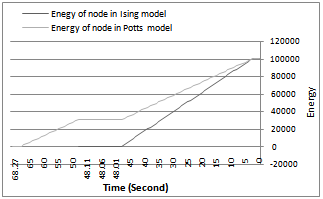 | Figure 5. Energy changes diagram for a node of the wireless network in Potts and Ising model |
5. Conclusions
In this paper, Potts model was utilized to increase wireless sensor network lifetime and to enhance objective tracking. Due to this model, three states are considered for each sensor node: active, inactive and standby. Each node is scheduled such that if a sensor node detects a target or becomes informed of passing a target by receiving a signal from its neighbours, it becomes active and informs other neighbours around itself of this event. Otherwise, if no event exists around the node, first it becomes standby and after passing some time, if no event occurs, it becomes inactive. The advantage of standby state is that when a node is in this state, not only it consumes less energy than active state, but also changes its state into active state much faster and with less energy than inactive state in case of an event occurrence. Therefore, it saves energy. In diagrams, it is observed that the number of standby states is more than of active states. However, with increasing w, that is by increasing the radius of sending packets, network lifetime decreases because of communication Increase in both models.Notes
1DELTA EQUAL TO: equal to by definition.
References
| [1] | I. F. Akyildiz, et al., Wireless sensor networks: a survey, Computer Networks, Vol. 38, pp. 393–422, 2002. |
| [2] | Abhishek Srivastav, Asok Ray, and Shashi Phoha, “Adaptive Sensor Activity Scheduling in Distributed Sensor Networks: A Statistical Mechanics Approach,” International Journal of Distributed Sensor Networks, 5: pp. 242–261, 2009. |
| [3] | Laura Beaudin, “A Review of the Potts Model: Its Connection to the Tutte Polynomial and its Application to Complex Experiments” Saint Michael’s College, 2007. |
| [4] | M. Vafaei Jahan, M.R. Akbarzadeh Totonchi, “Hybrid local search algorithm via evolutionary avalanches for spin glass based portfolio selection,“ Egyptian Informatics Journal, Vol. 13, Issue 2, pp:65-73, 2012. |
| [5] | M. Vafaei Jahan, “Multi Scale Spin Glass Based Portfolio Selection” Advances in Computing, No. 1, Vol. 2, pp:6-11, 2012. |
| [6] | Chang, Shu-Chiuan; Shrock, Robert. “Exact partition function for the Potts model with next-nearest neighbor couplings on arbitrary-length ladders.” International Journal of Modern Physics B, Vol. 15, No. 5, pp. 443-478, 2001. |
| [7] | Welsh, D. J. A.; Merino, C. “The Potts model and the Tutte polynomial. Probabilistic techniques in equilibrium and nonequilibrium statistical physics.” J. Math. Phys. Vol. 41, No. 3, pp. 1127-1152, 2000. |
| [8] | Jorgensen, William L. “Perspective on ‘Equation of state calculations by fast computing machines.” Theoretical Chemistry Accounts. Vol. 103, pp. 225-227. July, 1999. |
| [9] | G. R. Grimmett, ‘‘A theorem about random fields,’’ Bull. London Math. Soc., vol. 5, no. 1, pp. 81–84, 1973.[Online]. Available: http://blms.oxfordjournals.org. |
| [10] | D. B. West, Introduction to Graph Theory, 2nd ed. Prentice Hall, pp. 1-100, 2000. |
| [11] | K. Huang, Statistical Mechanics, 2nd Ed. New York, NY, USA: John Wiley, 1987. |
| [12] | P. Bouthemy, C. Hardouin, G. Piriou, and J. Yao, ‘‘Mixed-state auto-models and motion texture modeling,’’ J. Math. Imaging Vis. Vol. 25, no. 3, pp. 387–402, 2006. |
| [13] | Jinhua Guo, Weidong Xiang, and Shengquan, “Reinforce Networking Theory with OPNET Simulation”, Journal of Information Technology Education, Wang University of Michigan-Dearborn, MI, USA,Vol. 6, pp. 215-226, 2007. |
| [14] | J. Polastre, R. Szewczyk, and D. E. Culler, ‘‘Telos: enabling ultra-low power wireless research.’’ in IPSN, pp. 364–369, 2005. |
| [15] | J. L. Hill and D. E. Culler, ‘‘Mica: A wireless platform for deeply embedded networks,’’ IEEE Micro, vol. 22, no. 6, pp. 12–24, 2002. |
| [16] | http://www.digikey.com/us/en/techzone/sensors/resources/articles/low-power-wireless-sensor-networks.html. |
| [17] | V. Raghunathan, C. Schurgers, S. Park, and M. Srivastava. Energy aware wireless microsensor networks. IEEE Signal Processing Magazine, 19(2):pp. 40–50, March 2002. |
 Abstract
 Reference
 Full-Text PDF
 Full-Text HTML