1. Introduction

The functioning reliability evaluation of an industrial system in operating mode consists of analyzing failures component to estimate their impact on the service provided by the system [1], [2] and [3].

A particularity in characterizing a number of industrial systems is that their behavior varies as function of time due to interactions between components of the system or as function of the environment. Thus, we are talking about dynamic reliability [4], [5], which render conventional methods of functioning reliability static and ineffective. According to [6] the dynamic reliability is the predictive evaluation reliability of a system, whose reliability structure expresses how the system failure depends on the failures of its components, evolves dynamically over time.

Thus, an industrial system will evolve physically over time in nominal operation, in a degraded or failed mode. The maintenance and the process organization which allow the functioning of a system will have an impact on its performance.

In general, the efficiency evaluation of the maintenance action can be done by estimated methods based on feedback experience knowledge or Bayesian methods based on expert opinions [7], [8].

Bayesian networks (BN) are based on graph theory and probability theory. They allow to represent intuitively systems whose state evolves in a non- deterministic manner [9]. In addition, they have the ability to integrate in the same model various kinds of knowledge (Rex, expertise and observation).

However, the BN formalism does not allow to represent systems evolving over time i.e that contain variables whose conditional probability table (CPT) in present time which depends on past information [10], [11]. This problematic type led us to use dynamic Bayesian networks (DBN). The DBN are an extension of BN which model a stochastic processes varying over time. In addition statistical nodes used in conventional BN, DBN introduce a new type of nodes called temporal nodes to model discrete random variables depending on time [12], [13] and [14].

The objective of this paper is to evaluate the system reliability without maintenance intervention, then show what will be the efficiency of the maintenance strategy of the same system.

The performance evaluation model for a maintained system involves the following steps:

- modeling the system from its topo-functional decomposition in components,

- modeling the degradation modes of various components,

- modeling functional dependencies between components and their effects on the process of the system by measuring the safety parameter,

- identification and incorporation of maintenance strategies and system performance evaluation.

2. Bayesian Approach for a Degradable System

The degradation of a system can be considered according to various modes. It is suggested to consider them according to the following two situations: the system is not maintained (only a few corrective maintenance operations are realised) or the system is maintained according to predefined maintenance strategy.

The topology describing the degradation of a component is shown in Figure 1 [9], [10], [15], [16].

Figure 1. Topology Describing Degradation Component

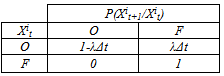
The sequence (X_t), 1 ≤ t ≤ T, is the system state on a sequence of length T. In this graphical structure, it is necessary to define the table of conditional probabilities allocating the probability to see the component (system) changing from state to state. In this phase, two groups of components are to be distinguished: the components at constant failure rate, and those with variable failure rate:

• Components at constant failure rate:

The set values of variable is val, in this case we should determine only the conditional probabilities:

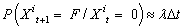
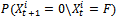indicates the probability that the component passes naturally from the failure state to the operating state for non-auto repairable systems. It is equal to zero.

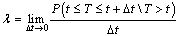
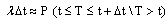
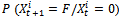indicates the probability that the component state degrades over time period Δt separating the decision instants t & t+1. This means that,

(1)

Where: T is a random variable absolutely continuous and strictly positive which represents the period before failure. To determine the value of P(t≤T≤t+Δt\T>t), we must first restate the definition of failure as.

(2)

So, if λΔt is small, Eq. 2 becomes

(3)

Using Eq. 1, the conditional probability P(Xⁱ_t+1= F/Xⁱ_t= 0) is given by:

(4)

The term λΔt can be seen as the probability that the system is failing in the interval [t, t +1]. Finally, and to simplify the estimation of the variable, the CPT of the node is written as follows:

Table 1. Conditional Probabilities Table (CPT)

• Components at variable failure rate:

DBN structure remains the same, but its parameters are distinct. Indeed, the network will have two nodes Xⁱ_t and Xⁱ_t+1 of the random variable in two successive time steps which is the set of values, val {Xⁱ}= {0, D₁, …… D_Nd , F}.

Where: D_j, j∈ [1, N_d] are a set of states in series, geometrically distributed, N_d is their number.

(5)

Then, this network is completed by introducing the functional dependencies describing the reate degradation of one component as function of the state of its neighborhoods.

To model the dependence components C_i and C_j, it is sufficient to join nodes X^j_t to Xⁱ_t+1 (Figure 2).

The CPT of node Xⁱ_t+1 has the following form:

Table 2. Conditionnel Probabilities Table (CPT) of node Xit+1

The CPT of node Xⁱ_t+1 is duplicated and its dimension increases with the number of dependencies.

From this analysis, it is possible to consider the planned maintenance actions and follows the behavior of the system. Maintenance strategies may be different but correspond on intended influences brought on the system. A maintenance action is used to modify the intrinsic trajectory of the degradation of the system state. The strategy elements considered in this study concern only the performed tasks, particularly their effects on the functioning of each component of the system.

Figure 3 shows the general layout of the proposed model.

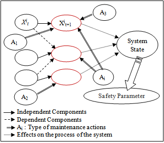Figure 3. General Layout of the Model

3. Industrial System Description

Analysis of real case study with and without maintenance described above was applied to a Blower of a lemonade production line.

Figure 4 shows the production line of soft drink for formats 0.5l or 2l depending on the configuration of the machines. At the input line, there are the raw materials appearing in preform and at the output line we get packaged bottles on pallets to be transferred to the stock.

The blowing process consists of the following phases:

• a heated preform is placed in the open blow mold,

• the blowing mold closes, the elongation rod move gradually, first in the transport chuck then, when the blowing mold is locked, into the preform up to its ends,

• the joining piston connects tightly to the chuck transport,

• when the elongation rod reaches the end of the preform, blowing air P1 is switched ON through a high-flow valve. A limited supply of P1 allows to control the formation of the "bubble bottle" and thus a homogeneous distribution of the material,

• the blowing pressure P1 is deactivated and the blowing pressure P2 is activated, the bubble bottle is pressed onto the mold wall with a higher pressure. This system allows the finest contouring of the bottle,

• the blowing process is complete when the blowing air P2 is cute through the high-flow valve P2 and when the blowing air is discharged through the piston and the high flow valve in the silencer,

• the connecting piston is downed, the blowing mold is unlocked and opened, and the finished bottle is extracted from the opened blowing mold.

In this production line, the Blower is taken as a case study because of the following reasons:

• the high frequency of failure of this machine,

• the technology complexity of the machine,

• the machine maintenability.

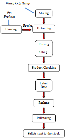Figure 4. Production Line of Soft Drink Manufacturing Process

We not that this equipment has only a few operations of corrective maintenance.

The decomposition of the machine in components is as follows:

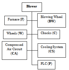Figure 5. Blower Decomposition

4. Modeling and Simulation of a System Functioning Mode

4.1. Behavioral analysis of system components

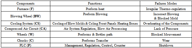
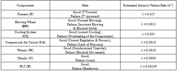
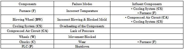
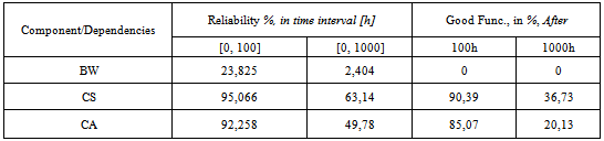
To simplify the analysis of the components behaviour, in the first step are analyzed separately and then treated according to their mutual dependencies, given that initially the system is not maintained.

For each component the function and the failure mode are defined as shown in Table 3.

Table 3. Function and Components Failure Mode

The various components states and their intrinsic failure rate are given in the Table 4. The intrinsic failure rate determination is mainly from the history of failures and calculated by the formula given by Eq.6.

(6)

Where the MTBF is the mean time between failure.

Table 4. States and Components Intrinsic Failure Rate

As an example of the analysis process, we describe in the next figure the model representing the evolution of the component state of the "Furnace", considered separately from other system components, in the time interval [t to t +1].

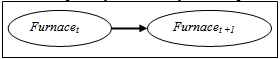Figure 6. Degradation Indication Topology of the Furnace

The same approach is used for the other components listed in Table 4.

Consequently, the obtained Conditional Probability Table is given in Table 5.

Table 5. Conditional Probability Table of Node Furnacet+1

For a time interval (Δt) equal to 1 hour, the behaviour evolution of the Furnace is given in Figure 7.

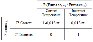
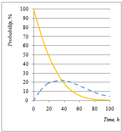
Figure 7. Dynamic Evolution Probability of the Furnace Good Functioning

The good functioning of the Furnace is conditioned by the temperature at the preform which should be at 117°C and 6°C. But in graph given by Figure 7 the probability of maintained good temperature is only 7.585% over the interval [0, 1000h]. This is explained largely by the recurring problem of the ignition of infrared lamps and burners.

More precisely, the component state can be characterized by several degradation regimes depending on the state of other elements that are linked to the same system.

In this case, the functional dependencies are listed in the Table 6.

During the blowing process, the Blowing Wheel must be supplied with compressed air (for preforms blowing) and with water (for cooling), in this case, the state of the Wheel depends on the Compressed Air Circuit and Cooling System. Therefore, the probability that blowing process is carried out depends on the intrinsic probability of failure of the Blowing Wheel and also on the probability of the states of its two associated components.

Table 6. Functional Dependencies Components

The model given in Figure 8 shows the state evolution of the Blowing Wheel in the time interval [t to t+1] with its functional dependencies represented by the arcs in dotted lines.

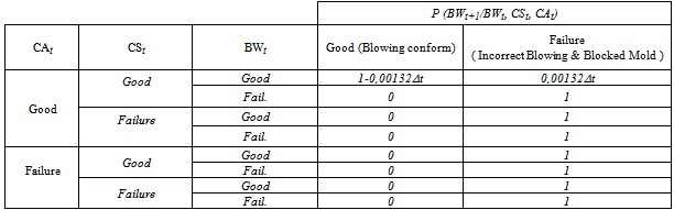
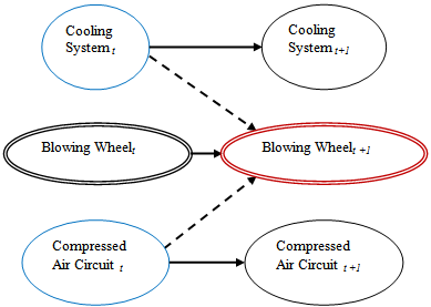Figure 8. Topology Indicating the Blowing Wheel Degradation with its Functional Dependencies

For this configuration, the table indicating the conditional probabilities of the Blowing Wheel is given Table 7.

Table 7. Conditional Probabiliy Table of Blowing Wheelt+1

The value 0.00132Δt corresponds to the Blowing Wheel failure probability by considering its dependencies effects characterized by the degradation probability of the Compressed Air Circuit and the Cooling System. Thus, from the estimation Eq.6 we can deduce various degradations effects mechanisms of the influent components, estimated at 10% of the calculated value.

Other probabilities are equal to 1, because if the Compressed Air Circuit and/or Cooling System fail at instant t, the blowing at t+1 will not be conform.

For a time interval (Δt) equal to 1 hour, the evolution behaviour of the Blowing Wheel component and its various dependencies (Compressed Air Circuit and Cooling System) studied on two time intervals [0, 100 h] and [0, 1000 h] is shown in Figure 9 and Figure 10.

Figure 9 and 10 show the probability variation of good functioning and reliability on [t, t+n] interval of the Blowing Wheel (curve C3) based on its two dependencies: Cooling System (curve C1) and Air Circuit (curve C2).

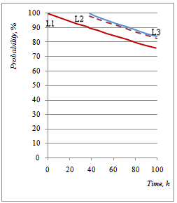
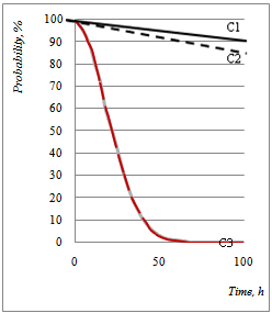Figure 9. Evolution of the Dynamic Probability in Good operation of the Blowing Wheel and its two dependencies in [0,100h] interval

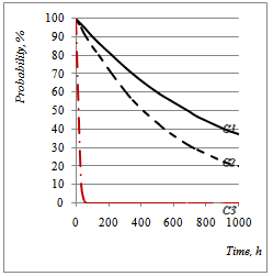Figure 10. Evolution of the Dynamic Probability in Good operation of the Blowing Wheel and its two dependencies in [0,1000h] interval

The reliability values are given in Table 8.

Table 8. Reliability Values and Good Functioning

From these results, in the considered time intervals, it is easy to see that the Blowing Wheel has very low reliability and poor functioning rate. This performance decrease is accentuated even more with the degradation of Cooling System and Compressed Air Circuit. Resulting in an alteration of the whole blowing process.

To constitute the global network, in the same manner, we carry out the state analysis of the Furnace and Chucks components according to their dependencies (Table 6) and their influence on the machine state. This state was determined by the machine functional analysis allowing the identification of three states: Normal Functioning, Shutdown, Degraded Functioning (with scrap), as indicated in the table below.

Table 9. Component Effect Failure on the Machine Components Component Effect Failure on the Machine Furnace (F) Degraded Functioning Blowing Wheel (BW) Shutdown Cooling System (CS) Degraded Functioning Compressed Air Circuit (CA) Degraded Functioning Wheels (W) Shutdown Chucks (C) Shutdown PLC (P) Shutdown

From these considerations, the model can be represented in the following topology (Figure 11).

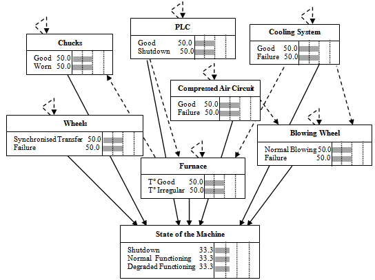
Figure 11. Proposed Model Topology

4.2. Network Architecture Conception

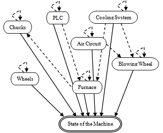
The equivalent network architecture was developed under Netica software, before taking into account maintenance strategies.

Each input node indicates a machine component.

The solid lines are synchronous arcs, and they represent the relationship between components and machine state.

Figure 12. Proposed Model without Maintenance

The dotted lines are diachronic arcs, they represent the evolution behavior of various components with their functional dependencies.

Figure 13. Global Modes Network

The model configuration, presented with the associated modes to various nodes is given by Figure 13. These modes represent the various possible states of variables in the network.

To test the global operation network, we take as a time interval time (Δt) = 1 hour. The simulation is performed in several steps of 9 steps each. The results of each completed step are considered in their turn as an input values to the next step, however it should be noted that this approach leads to a slight decrease in accuracy. The results are presented in Figure 14.

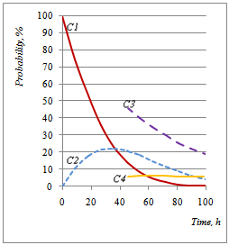
Figure 14. The Dynamic Probability Evolution of Good Functioning of the Blower and Scrap Rate

The first curve (solid line) shows the decreasing evolution probability of the Blower in good functioning. Indeed, if the equipment is functioning permanently and without maintenance, it becomes prone to a more or less rapid degradation (aging) which can lead to partial or total failure.

The second curve (dashed) corroborates this observation, the scrap grow significantly, this is due to the lack of maintenance (different systems do not provide the same performance). The maximum recorded value (22%) of the scrap rate falls to a state of the equipment in the critical area, much below the alert zone which call for the maintenance intervention. From this point on the material has no longer the ability to perform its required function and any manufactured product meets no longer the standard quality.

The next step is to include in this model the maintenance actions according to the different possible strategies. To this end the following actions are considered:

• the actions (preventive and/or corrective) with possible effects on degradation mechanisms and failure modes, depending upon the decision to replace all or part of the failed hardware,

• the maintenance actions are assumed to be perfect. The executed action at time t on the component produces automatically and definitely an effect at time t+1.

It is recognized that maintenance action, should at least keep the material in the condition that was before failure occurrence. Thus, evaluating the effectiveness of the various action types consists in estimating the parameter ρ as given in Table 10 (next page).

Table 10. Maintenance Efficiency Tasks After Repairing State

By convention, it was decided that the choice of action type is limited to its ability to be applied to the major cause of component failure and to assess its effect on the machine behavior.

The action types associated to components is shown in Table 11, where X indicates the relevant type of action that a given component is prone to undergo.

Table 11. Action Types Associated to Components Components AGAN ABAO ASGO Furnace X Blow Wheel X X X Cooling System X X X Compressed Air System X X X Wheels X X X Chucks X X X PLC X

For components, Furnace and PLC, the action types ABAO and ASGO are not applicable, since their main failures are instantaneous and require changing equipment.

The model in Figure 15 represents the evolution state of Wheels at instant [t to t+1], taking into account the effect of recommended maintenance actions.

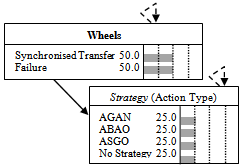Figure 15. State Evolution Model of Wheels Taking Into Account its Associated Maintenance Action

Thus, the obtained conditional probability table of this model is given in Table 12.

Table 12. Conditional Probability Table of Wheelst+1 Node P (Wheelst +1/ Wheelst , stratégies) Stratégies t Wheelst Good Defect AGAN Good 1 0 ASGO 1 0 ABAO 1-0,0028t 0,0028t No strategy 1-0,0028t 0,0028t AGAN Defect 1 0 ASGO  0,2 ABAO 0 1 No strategy 0 1

The data in Table 12 reveal the impact of maintenance actions according to the recommended strategy and we can observe that:

- if the selected action type at instant t is of type AGAN, the probability of good functioning at t+1 is 1,

- for the ASGO type, there are two possibilities: the Wheels are in good functioning and the good functioning probability at t+1 is equal to 1 or the Wheels are in default and their probability is ρ (in this case, the type ASGO effectiveness is estimated at 0.8),

- and finally, for the type ABAO, the Wheels follow their natural degradation with a failure probability of 0.0028 Δt.

For a time interval (Δt) equal to 1hour, the behavior evolution of Wheels is described in Figure 16.

Line L1 represents the Wheel degradation due to insufficiency (or inefficiency) maintenance interventions (ABAO type). It is easy to see that this degradation for the chosen time interval follows a natural evolution.

Figure 16. Dynamic Probability Evolution of Wheels in Good Functioning Mode Based on Possible Strategy of Maintenance

The two other lines show where the Wheel state evolution is depending on the chosen strategy. However, in this case, it turns out that the maintenance effects actions of the two strategies (AGAN and ASGO) on Wheels are almost identical, their efficiency bring better Wheels behaviour. In both cases, the maintenance intervention will only occur when the probability of good functioning reaches 90% at t=37 hours.

In Figure 16, the representation of AGAN and ASGO lines start at t =38 hours, which correspond to their starting effect (i.e. t+1 of instant t=37hours).

When this approach is applied to other components it leads to the design of the global network by integrating various degradation models in highlighting all the components involved and their adopted maintenance strategy.

Synchronic arcs are shown as solid lines, in Figure17 while diachronic arcs are symbolized by dashed lines.

The final choice between the two strategies will depend on subsequent maintenance costs, the general maintenance policy and so on.

The model given in Figure 18, defined modes of different nodes. They indicate the various possible states that the network variables can includ.

The distinctions are:

- for components and machine: modes provide information on their operating states,

- for maintenance strategies: the modes tell about various kinds of actions that the components are prone to undergo.

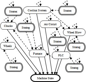Figure 17. Global Model Architecture

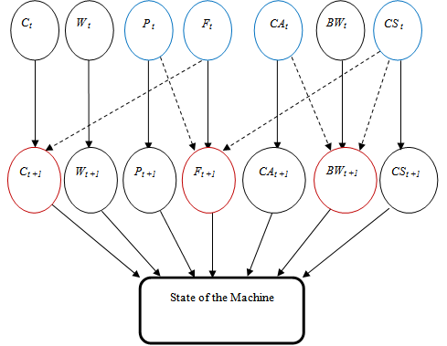
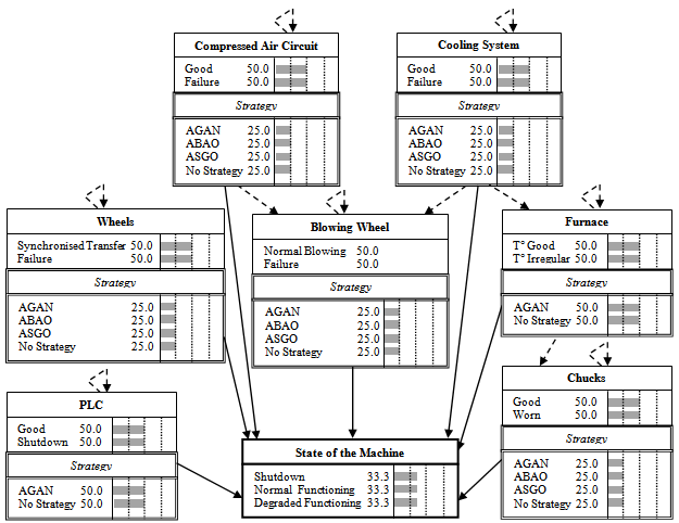Figure 18. Topology Representing the Nodes of the Global Model

The time interval (Δt) is considered equal to 1hour. To exploit the network results, and show the interest of this approach, we present an example to evaluate safety parameters while taking into account the maintenance strategy.

In this example we determine the functioning probability of the Blower, applying AGAN maintenance on the Wheel and Blower, the Furnace at time t = 45 hours.

The obtained graph is given in Figure 19.

Figure 19. Dynamic Probability Evolution of the Blower Good Functioning with the Applied Strategy

In the absence (or insufficient) of strategy maintenance on the Furnace and the Blower Wheel, the Blower will undergo a significant and persistent degradation which can lead to total failure. There are multiple reasons, but inexorably, the behaviour of these two components of the machine is strongly influenced by the status of the other components which are the Cooling System and the Compressed Air Circuit. If these last components, with their high criticality, are not maintained the degradation of the Blower will be severe. This observation is validated by the curve C1 which shows clearly the rapid degradation of the physical state of the Blower with the consequent increase in the scrap rate C2. If after 45 hours, the scrap rate tends to decrease it is only because of the slowdown (may be the Shutdown) of the machine.

Using appropriate maintenance actions on the concerned elements, the state situation of the Blower is better, with a delayed degradation and better control (C3). The scrap is much more reduced and stabilized (C4).

4.3. Application

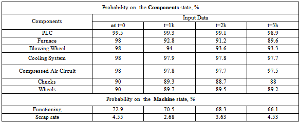
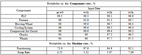
The performed simulations with this network, without any architecture modification and conditional probabilities tables, in various scenarios (diagnosis, predictions and combined reasoning) allows to show the efficiency and flexibility of this tool as a decision tool.

If, wish for example, to establish a prediction of the maintenance strategy impact, simply insert the input nodes values of the components according to their estimated state at instant t and the appropriate maintenance strategy. Informed input nodes automatically update output nodes from t to t+n.

The approach consists in comparing the state evolution of the machine with and without maintenance strategy.

If no maintenance action is considered (strategy = 0) and considering the components at t = 0 are in good state, thus the obtained results are given in Table 13.

Table 13. Prediction of the State Machine Evolution without Maintenance Strategy

It is easy to see a degradation of all components having as consequence a faster deterioration of the machine state and an increased scrap rate.

On the other hand, providing a maintenance strategy of type ASGO at t = 0h for predisposed items (Blowing Wheel, Cooling System, Compressed Air Circuit, Chucks, Wheels), components degradation is less significant with better behaviour of the machine. The increased scrap rate registered is probably due to the fact that no maintenance of the Furnace is provided (Table 14).

Table 14. Prediction of the State Machine Evolution with Maintenance Strategy

5. Conclusions

In this paper, a model is developed for a system behavioral analysis by considering the degradation modes of various components some of which may be interrelated and have variable behaviours and unwanted, influencing later on the physical evolution of the entire system. Then in the final architecture of the model were incorporated types of maintenance strategies and their reciprocity efficiency.

The attempts in the design of the model we have taken to the ration of a flexible architecture for its various applications and easy to implement.

Throughout the presented example, we illustrate the approach usefulness and its use as part of a process for predictive evaluation of the safety parameters of a system in operating modes and the effects of maintenance strategies. The network learning was realized by exploiting the data obtained from various sources (expert opinions, historical).

Other possible use is that the model can serve to plan the actions of maintenance by giving the periods and the natures of the intervention of a way anticipated according to the constraints in terms of objectives of performance. That is be able to envisage in a simultaneous way the nature of the action as well as its moment of execution. In that case, the strategies of maintenance will thus be designed by a set of couples (time, action), what constitutes a tool of reliable decision for the managers of maintenance. This aspect we continue to develop it by including other variables such as the costs associated to each strategy of maintenance, the protocols of the interventions etc…

ACKNOWLEDGEMENTS

The author would like to thank Prof. Ahcene SERIDI for reviewing the final manuscript.