1. Introduction

The hardware developments from recent years have made multi-core architectures a common place in the industry. The issue we are now facing is taking advantage of such platforms.

Parallel and distributed versions of the genetic algorithms (GAs) are popular and diverse. The simplest parallel models are function-based where the evaluation of the fitness function is distributed among the processes[14]. The most popular parallel models are population-based where the population itself is distributed in niches[15], also called islands sometimes[9]. Such models require a periodic migration of individuals between the sub-populations. Theshared-memory GAs are a subset of the parallel and distributed models. The parallelization techniques can be ported and adapted from one type of architecture to the other, but with specific features that can be optimized in each case. A survey of these algorithms can be found in[1].

There are positive arguments in favor of models based on population division, such as a high degree of independence for each process. Among the drawbacks we can cite the fragmentation of the population into small pieces. This can generate issues such as the premature converge of the population to a local optimum or general loss of diversity. Larger populations have been reported to perform better by several studies or even to be necessary to the success ofparallel implementations[3].

In a different direction, coevolutionary algorithms have interested and fascinated researchers for a good number of years. Even though competitive coevolution is the more popular form, the cooperative form has been proven to give good results[2]. These approaches decompose the problem into parts evolving separately[12]. For the purpose of the fitness evaluation, these parts are assembled into a complete chromosome.[7] argues that it is not the separability of the problem that makes these approaches successful, but their increased exploratory power. Some theoretical studies of the conditions under which these algorithms can achieve the global optimum have been proposed[10].

The model that we propose in this paper bridges the gap between these two approaches. It is a variant of the cooperative coevolutionary approach designed for shared memory parallel architectures. While the usual cooperative approach is implemented for problems that are naturally divisible into subpopulations, our model generalizes this technique by making it applicable to any problem.

Our model is based on a division at the genotype level of the population into several agents or processes. It is not an algorithmically equivalent version of the genetic algorithm, or of a standard cooperative coevolutionary algorithm, but a hybrid model designed for parallel architectures. This model can potentially run faster and achieve better results than the standard GA. In our approach, each process receives a partial chromosome to evolve. All the genetic operations are restricted to this subset of genes. For evaluation purposes, a template is kept by every process containing information about the best genes found by all of the other processes up to that point. A periodic exchange procedure keeps this information up to date.

Finally, when aiming to optimize the genetic algorithms for massively parallel architectures, it becomes undesirable both to split up the population into too small nests, and to divide the chromosome too much. A hybrid approach can be a good compromise and for this purpose both population and chromosome division models need to be studied thoroughly. This paper contributes to the study of the less observed of the two approaches.

The paper is structured the following way. Section 2 presents the details of our parallel model for the genetic algorithms. Section 3 introduces the three test problems that we used for out experiments. Section 4 shows the experimental results and the paper ends with conclusions.

2. Chromosome Division Model

Our model for parallel genetic algorithms follows a similar idea to the one described in[16]. The difference is that the current model is implemented for shared memory architectures as opposed to a Beowulf cluster, and the experiments use a different set of problems. Preliminary results were also presented in[17,18], although the set of problems used here is almost entirely new.

2.1. Problem Division

According to the most popular approach to parallel genetic algorithms, which is the island one, the population is decomposed in several islands or niches, each of them evolving in parallel. In such a model, the evolution in each population is self-contained, and the only thing that makes it a unified process is an occasional migration of individuals between the islands.

Our motivation comes from the fact that smaller populations can more easily lead to suboptimal solutions and premature convergence. The chromosome division allows us to maintain a larger population for each process using the same amount of memory.

The idea behind this parallel model is that the problem to be solved is divided into several tasks. Each task is then assigned to a different process that will focus on it while exchanging information with the other processes. This is similar to a multi-agent approach that has been proved efficient for many applications before, in a variety of contexts.

Thus, in the approach proposed in this paper, the division happens along the genotype. The genes composing each chromosome are divided among the processes, such that the task of each process consists of evolving a pre-determined part of the chromosome. Each process performs the standard genetic operations on its subset of genes. When the fitness evaluation is needed, the subset of genes is inserted into a global template that allows it to be seen as a complete chromosome, as shown in Figure 1. The top chromosome in this figure represents the template, which is a chromosome with some missing genes. The pieces marked as “Population for P₁” represent partial chromosomes that complete the genes missing in the template. They are assembled together into a complete chromosome that can be evaluated with the usual fitness function. This template is periodically exchanged between the processes.

Our intention was to develop a model that can be applied regardless of the separability of the problem, but the test problems we chose are also designed to show how this aspect influences the fitness performance and the speedup.

All the genetic operators are performed according to their standard definition, with the exception that they are restricted to the subset of the genes assigned to each process.

Let n be the size of the chromosome, with the indexes for the genes going from 0 to n-1. Let us suppose that we have p processes. Each process will receive a part of the chromosome of size n_p = n/p. Then the process or agent with identity number id, 0 ≤ id ≤ p-1 will be in charge of the genes in the interval[id*n_p, (id+1)*n_p - 1].

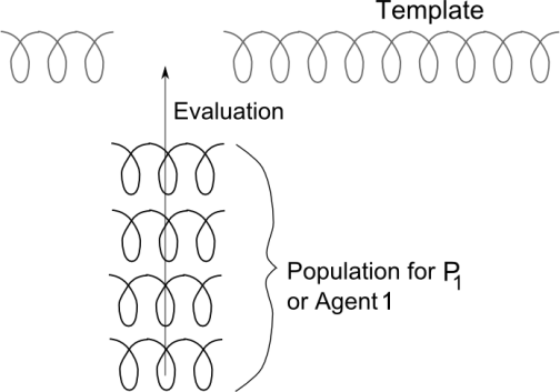Figure 1. A template for the population evolved by one of the agents

Practically, the chromosomes are stored for each process in two local collections representing the previous generation and the new one to be constructed from it. These collections are swapped after the completion of each new generation in a manner that is similar to the double buffer model in OpenGL. Thus, the most efficient way to handle the template is to copy it over all the chromosomes in both of these collections leaving out the genes of indexes assigned to the current process. This way, even though the genetic operators are localized, the fitness evaluation can proceed directly to the evaluation. The memory use in this procedure can be improved, by actually storing only the pieces of chromosomes assigned to each process, but that is not necessary unless we deal with a very large population and / or very large chromosomes.

The mutation operator is not affected by the chromosome division, and neither is the fitness-proportionate selection. The crossover makes our approach algorithmically different from the sequential one. With a one-point crossover as the base operator, each process chooses a crossover site within the range assigned to it. Thus, with 2 processes our overall operator is partially equivalent to the 2-point crossover. The second and more important difference with the sequential one is, though, being able to evaluate the quality of parts of the chromosome separately and have better chances to achieve a good solution overall.

We have used a 1-point crossover with probability 0.8 and a classic mutation with probability 0.01. The reproduction form is elitist for each process, preserving a single best chromosome from one generation to the next. Thus, even though the new template replaces the old one after each exchange phase, the new genes are either identical to the old ones, or proven to perform better.

2.2. Fitness Evaluation

There are a good number of benchmark fitness functions for genetic algorithms that are separable, meaning that they can be divided into sub-problems such that the evaluation of each of them can be accomplished independently. Our model is not restricted to these types of problems specifically, but is rather designed in a general way so that it can be applied to any fitness function. However, the evaluation procedure can be optimized for separable functions and a greater performance can be achieved in terms of execution time and use of each CPU core. One of out test problems will showcase this situation.

We start with the assumption that to evaluate the fitness function for any combination of genes, we need a full set spanning from 0 to n-1. Thus, to evaluate a partial chromosome, we need to complete it with the template. The evaluation consists of plugging the partial chromosome into the common template, and then passing this complete individual to the fitness function.

An exchange procedure insures that the template is kept reasonably up to date with respect to the latest best performing genes obtained by each process. During the exchange phase, each process copies the genes of the best chromosome found so far in terms of fitness to a global “best chromosome” shared by all the processes. After all of the processes have finished this update, each of them updates its own template from the global best chromosome. This procedure takes place periodically and can involve a synchronization of the processes in terms of number of generations produced in between the exchanges. Since only one chromosome is exchanged in the process, our model is coarse-grained. The next section talks about this aspect more in detail.

2.3. Synchronous vs Asynchronous Exchange

The only communication between the processes happens during the exchange procedure. From a synchronization point of view, we propose to compare two approaches. In the first one, each exchange phase happens after the exact same number of generations for each process, and this is accomplished through a barrier call. In this model, called synchronous, all the processes evolve approximately at the same time and during the exchange they need to wait for all of them to reach the entry point in order to proceed. The genes in each chromosome represent a fairly homogeneous evolutionary step during the fitness evaluation.

In the second approach, called asynchronous, each process can update the global best chromosome periodically without having to wait for any of the others. Thus, genes evolved in substantially different generations are combined for the evaluation of the fitness.

The synchronous exchange procedure is shown below in C++ based pseudo code. In this algorithm we assume that the indexes in the partial chromosome are kept consistent with the position of the genes in the complete chromosome. To make the procedure easier to understand, the id of the process is used as an index for the best partial chromosome and for the template. Practically, our implementation is object oriented, the exchange function is a class method, and these variables marked with the id are class attributes. The global variables shared by all the processes are shown with capitalized names.

void Exchange_synch(int id) {

np = Chromosome_Size/ Number_Of_Proc;

Barrier(Number_Of_Proc);

for (i=id*np; i<(id+1)*np; i++)

Best_Chromosome[i] =

best_partial_chr[id][i];

Barrier(Number_Of_Proc);

for (i=0; itemplate[id][i] = Best_Chromosome[i];

for (i=(id+1)*np; itemplate[id][i] = Best_Chromosome[i];

}

We can see below the asynchronous version of the exchange procedure where each process updates the best chromosome and its own template periodically without having to wait for the others. All the name conventions are the same as above.

void Exchange_asynch(int id) {

np = Chromosome_Size/ Number_Of_Proc;

Lock(&Mutex); // Write phase

for (i=id*np; i<(id+1)*np; i++)

Best_Chromosome[i] =

best_partial_chr[id][i];

Unlock(&Mutex);

Lock(&Mutex); // Read phase

for (i=0; itemplate[id][i] = Best_Chromosome[i];

for (i=(id+1)*np; itemplate[id][i] = Best_Chromosome[i];

Unlock(&Mutex);

}

The population is initialized for each process randomly, as it is usually the case. The template is initialized by calling the function exchange before the evolution process starts.

The exchange takes place every few generations, 10 for most of our experiments. Another question we will attempt to answer here is how much this exchange period interferes both with the execution time and with the performance in terms of best fitness achieved.

3. Test Problems

We have chosen three problems to test our parallel model with, two of them being of the benchmark type, and one a real-world problem. The specifics of each of them should allow us to showcase different features of our program. The benchmark problems consist of fitness functions of linear complexity over the number of genes and also uniformly fast to compute.

The real-world problem is computationally more expensive and non uniform over the set of chromosomes. For this last function, a global optimum is not known.

The two benchmark problems are chosen with a fitness that is linear over the chromosome length to show the speedup potential of our model for the most common category of problems. These functions are very similar to other problems used for benchmarking in various studies. The real-world problem is a difficult one chosen to showcase the potential of our model in terms of quality of solutions.

A second aspect that differentiates these problems is the reciprocal influence of genes at different locations in the chromosome in the computation of the fitness or separability. For the real-world problem, such influences are present, and a good performance cannot be achieved in the absence of proper process coordination. For the first benchmark problem, there is an even higher degree of reciprocal influence of the genes from one process to another than for the real-world problem. For the second benchmark problem the fitness influence is localized to the genes assigned to each process, meaning that this function is highly separable, and the algorithm is optimized to take advantage of it. Thus, we hope to show how our model can behave in each of these three situations.

For reasonable comparison grounds for the three problems we have used the same experimental settings as much as possible: population size (50), number of generations (1000), and chromosome size (360). The number of genes is determined by the number of parameters defining the real-world problem, and we were able to configure the two benchmark problems with the same value.

3.1. Benchmark Problems

The first problem is known in the literature as the Rosenbrock function[8,13] or the DeJong function[6], and as a difficult optimization problem. It consists of minimizing the following function:

(1)

where -1.5 ≤ x, y ≤ 1.5 for our experiments.

The minimum of 0 is achieved for x = y = 1. The difficulty of this function is that local minima with x = y are relatively easy to achieve, but both variables need to move towards the value 1 at the same time to find the global minimum. For this problem, the first half of the genes represents the value of x and the second half the value of y. Thus, in the parallel mode, the processes will be highly dependent on each other to achieve a good performance, which is the reason for choosing this function. For our experiments we have used 360 binary genes to be consistent with the two other problems.

The second function is of a category that has been used to test deceptive aspects of the fitness landscape[5]. This function maps each group of 3 binary genes in the sequence to a value based on Table 1 and then adds them up over the entire chromosome. This problem presents a difficulty to hill-climbing methods because the sequence of highest fitness, 111, is isolated from the suboptimal solution that is 000. Thus, the sequences that are close to the optimal solution are of low fitness, while those close to the suboptimal ones have a higher fitness, to mislead the algorithm. With a population size of 360, the optimal solution has a fitness of 3600 while the suboptimal one of 3360. Since the value of each set of 3 genes is computed separately from any other set of 3 genes, this fitness is entirely separable. We use this problem to show the speedup potential for highly separable functions.

Table 1. Mapping from sequences of 3 bits (1st row) to fitness values (2nd row) for the deceptive problem 000 001 010 011 100 101 110 111 28 26 22 0 14 0 0 30

3.2. Real-Life Problem

The third problem we are using consists of optimizing the parameters defining a pilot for a simulated motorcycle. For this problem, the evaluation requires significantly more computations, and thus it will allow us to observe the improvement in performance in that respect. Contrary to the linear functions, the complexity of evaluating a chromosome is not uniform, but can vary significantly from one individual to the next. This constitutes an additional challenge for the parallel model. This function is partially separable.

The physical model of the motorcycle has been more extensively described in[19] and is close to[4]. The motorcycle is modeled as a system composed of several elements with various degrees of freedom, consisting of position and orientation on the road, speed, rotation of the handlebars, and leaning.

The driver's input into the system is defined by the tuple u=(τ, β_f, β_r, φ, α) where τ is the acceleration in the direction of movement provided by the throttle/gear control, β_f, β_r are forces applied on the front and rear brakes respectively, φ is the leaning angle, and α is the handlebar turning angle. This driver can be either a human player or an autonomous agent controlling the vehicle.

The movement is defined by Newtonian mechanics, where the acceleration is defined by gravity, friction, drag, and the throttle. The brakes are factored into the friction force.

The autonomous pilot uses perceptual information to make decisions about the vehicle driving. This information consists in the visible front distance, the lateral distance to the border of the road from the current position of the vehicle and from a short distance ahead of the vehicle, and the slope of the road.

The motorcycle is driven by several control units (CUs), each of them controlled by an independent agent. The current CUs are the gas (throttle), the brakes, and the handlebar/leaning. Each of these CUs is independently adjusted by an agent whose behavior is intended to drive the motorcycle safely in the middle of the road at a speed close to a given limit. The agents behave based on a set of equations relating the road conditions to action. The full set of equations is described in[19]. The equations comprise a fair number of coefficients and thresholds, and these are the values that are evolved by genetic algorithms.

To apply the GA to this problem, we chose a representation where each configurable coefficient is assigned 10 binary genes, and the chromosome results by concatenating all of the coefficients. As we have 36 coefficients, the chromosome has a length of 360.

A chromosome is evaluated by running the motorcycle in a non-graphical environment once with the pilot configured based on values obtained by decoding the chromosome over a test circuit presenting various turning and slope challenges. Each run can end either by completing the circuit, or by a failure condition. A failed circuit can be caused by one of the following three situations: a crash due to a high leaning angle, an exit from the road with no immediate recovery, or crossing the starting line without having reached all the marks, as when the vehicle takes a turn of 180 degrees and continues backward.

To compute the fitness we marked 50 reference points on the road and counted how many of them were reached by the motorcycle with a given degree of approximation. The fitness is computed as follows:

(2)

where d_m is the number of points reached by the motorcycle, d_t is the total number of points, and t_m is the total time taken until either the circuit was completed, or until a failure condition was detected.

Thus the fitness reflects both what percentage of the circuit the motorcycle has completed, and how fast it was capable of finishing the track. In general, a fitness value that is higher than 1 indicates completion of the circuit.

This problem is partially separable in a subtle way. For the motorcycle pilot to be able to function at all, it needs reasonable values for the parameters defining all of its agents. Thus, the pilot could be using the gas pedal perfectly well, but if the steering is ineffective, it will still fail. Once we have reasonable values for most of the agents of the pilot, each of them can be improved separately. Thus, this is an intermediate problem for the study of this aspect.

4. Experimental Results

In this section we present some of the experimental results with our model testing both the executions time/speedup and the fitness performance. Table 2 introduces the platforms that we have used for our computations. In the operating system column, XP stands for Microsoft Windows XP, W7 stands for Microsoft Windows 7, OsX stands for the Mac OsX 10.5.6, and Ub stands for Ubuntu 8.04. The program was implemented in standard C++ using the pthread library and its local version for each platform. The code that is being run is the same on all of the platforms for each reported experiment.

For the experiments concerning the speedup, there is no point in comparing approaches that don't perform a comparable number of computations. Since the speedup is our foremost interest here, we have chosen to run all the experiments with the same number of generations.

Table 2. Technical specifications of the platforms used for testing Label CPU Make CPU Speed Cores OS U1 Intel Pentium 4 2.8 GHz 1 Ub M2 Intel Core 2 Duo 2.4 GHz 2 OsX MX2 Intel Core 2 Duo 2.4 GHz 2 XP X2 Intel Dual Core T7200 2.0 GHz 2 XP U2 Intel Dual Core T7200 2.0 GHz 2 Ub X4 Intel Quad Core Q6600 2.4 GHz 4 XP X47 Intel Quad Core Q6600 2.4 GHz 4 W7

A second factor needs explanation before we proceed: the population size. In our approach we can level the parallel model with the sequential one on only one of two aspects: the number of evaluations performed on the whole, or the number of genes generated on the whole. We have chosen to generate the same number of genes as in the sequential model for all of our experiments, which means running the experiments with the same population size. This is consistent with the fact that one of the goals of the chromosome division is to be able to run the evolution with a larger population for each island.

4.1. Synchronous versus Asynchronous Exchange

The first set of experiments compares the synchronous versus asynchronous exchange models on different platforms for a variety of number of processes.

Table 3 shows the average execution time as number of seconds for the Rosenbrock function. Table 4 shows the average execution time for the deceptive problem. The chromosome length is 360, the population is of size 50, and we have run 1000 generations in all the cases. The results are averaged over 100 runs. The column labelled “Com” identifies the exchange function as synchronous (S) or asynchronous (A).

Table 3. Timing in seconds of the Rosenbrock function in 1000 generations, average over 100 runs Platf. Com #Processes 1 2 4 8 U1 S 2.61 3.79 5.51 13.12 U1 A 2.61 2.80 3.57 5.15 M2 S 0.88 0.69 0.82 1.04 M2 A 0.88 0.63 1.17 2.22 MX2 S 1.19 0.74 1.47 2.75 MX2 A 1.19 0.73 1.01 1.56 X47 S 3.24 2.60 2.30 8.24 X47 A 3.24 2.66 2.26 4.20

To complement these timing results, Tables 5 and 6 show the speedup in all of these cases computed as the execution time on a single process divided by the execution time of each multi-threaded run. A speedup of more than 100% represents a faster execution time in parallel than sequentially. Note that the speedup for 8 processes is not expected to be improved on any of the platforms, since the maximum number of cores that were available on any of the machines is 4. This table shows that on most multi-core architectures, the execution time for a number of processes less than or equal to the number of cores presents a speedup.

Table 4. Timing in seconds of the deceptive function in 1000 generations, average over 100 runs Platf. Com #Processes 1 2 4 8 U1 S 2.19 2.65 5.61 13 U1 A 2.19 2.39 2.78 3.59 M2 S 0.59 0.57 0.66 0.89 M2 A 0.6 0.53 1.12 2.16 MX2 S 1 0.54 0.9 1.27 MX2 A 0.99 0.54 0.62 0.77 X47 S 1.96 1.23 0.88 4.68 X47 A 1.91 1.23 0.9 1.39

Table 5. Speedup for the Rosenbrock function computed as the sequential time divided by the parallel time Platf. Com #Processes 2 4 8 U1 S 68.87% 47.37% 19.89% U1 A 93.21% 73.11% 50.68% M2 S 127.54% 107.32% 84.62% M2 A 139.68% 75.21% 39.64% MX2 S 160.81% 80.95% 43.27% MX2 A 163.01% 117.82% 76.28% X47 S 124.62% 140.87% 39.32% X47 A 121.80% 143.36% 77.14%

Table 6. Speedup for the deceptive function computed as the sequential time divided by the parallel time Platf. Com #Processes 2 4 8 U1 S 82.64% 39.04% 16.85% U1 A 91.63% 78.78% 61.00% M2 S 103.51% 89.39% 66.29% M2 A 113.21% 53.57% 27.78% MX2 S 185.19% 111.11% 78.74% MX2 A 183.33% 159.68% 128.57% X47 S 159.35% 222.73% 41.88% X47 A 155.28% 212.22% 137.41%

Table 7 shows the timing in seconds for the motorcycle driving problem. The settings in terms of chromosome length, population size, and number of generations are exactly the same as for the linear functions, except that we only ran the GAs 10 times for this problem in each case, due to the length of time required. Even thought 10 runs may not seem like a large enough number, each of these 10 runs we report represents between 2 and 7 days of uninterrupted and exclusive computation time on each platform and thus for the measuring of the speedup we consider them sufficient.

Table 7. Timing in seconds of the motorcycle driving, 1000 generations, average over 10 runs Platf. Com #Processes 1 2 4 8 U1 S 1969.3 6488.0 13308.1 32031.9 U1 A 1969.3 11985.9 7140.5 42254.5 M2 S 1789.7 7459.4 8396.22 12882.0 M2 A 1789.7 4381.5 8058.3 5809.2 X2 S 1292.5 2922.7 9542.0 10301.3 X2 A 1292.5 1885.9 4215.0 12439.2 X4 S 2081.0 3054.7 5452.5 16955.7 X4 A 2081.0 5638.4 5156.4 13561.6

Since the evaluation itself can take a variable amount of time depending on how long the pilot lasts on the road before a failure condition occurs, we thought that a normalized measure for the time was necessary. For this purpose, we also recorded the total number of times that the function move was called for the motorcycle simulation during the evaluation. We can consider these calls to be basic operations because they require a uniform amount of time. Since the function move is called repeatedly until either a crash condition occurs, or until the vehicle finishes the track, it is the number of such calls that introduces such variety in the evaluation time. Thus, this measure tells us the number of operations executed in every case.

Table 8 shows the number of such calls divided by 10⁴ as an average over 10 runs. For measuring the fitness obtained by each model, the platform is not important since the same code is run each time and we can thus average the results over 50 runs each for each parameter setting.

Table 8. Total number of moves for the motorcycle driving, divided by 104, average over 10 runs Platf. Com #Processes 1 2 4 8 U1 S 18678.0 4181.0 5849.6 11063.8 U1 A 18678.0 7080.8 5009.3 14515.9 M2 S 1882.0 6578.6 7344.5 13074.5 M2 A 1882.0 3732.1 7026.5 10269.1 X2 S 2063.6 5856.7 18086.0 19882.9 X2 A 2063.6 3993.2 8612.4 22640.5 X4 S 4051.3 7763.6 5942.9 14961.2 X4 A 4051.3 12176.1 5037.2 10394.8

Based on Table 8, we can now compute a normalized speedup by first dividing the execution time by the number of moves. The results of this operation are shown in Table 9. Then Table 10 shows the speedup for this problem by dividing this new timing measure for the sequential case by its value for the parallel case. From Table 10 we can see that the speedup achievement is lower for this problem than for the benchmark problems. This is due to the non-uniformity of the fitness calculation. Thus, the fastest process may need to wait for a long time for the lowest one to finish its task. Using an asynchronous model only improves the speedup for 8 processes on most platforms, which is contrary to the behavior observed on the benchmark problems. This can be explained by the improvement of the fitness achieved, since the better the pilot is, the more time it will be driving on the track without crashing. Even for this difficult problem, the parallel model makes good use of the multiple cores.

Table 9. Normalized time: computational time in seconds for 104 moves Platf. Com #Processes 1 2 4 8 U1 S 1.05 1.55 2.28 2.90 U1 A 1.05 1.69 1.43 2.91 M2 S 0.95 1.13 1.14 0.99 M2 A 0.95 1.17 1.15 0.57 X2 S 0.63 0.50 0.53 0.52 X2 A 0.63 0.47 0.49 0.55 X4 S 0.51 0.39 0.92 1.13 X4 A 0.51 0.46 1.02 1.30

Finally, we need to observe the average fitness achieved after 1000 generation for all the problems to see if the parallel model can perform as well as the sequential one in terms of quality of solutions or even better. Table 11 shows these results for all three functions, as an average of all the experiments performed on the various platforms presented in the timing tables. For the Rosenbrock function smaller values are better, while for the two others larger values are the goal.

We can see that the parallel model outperforms the sequential one in terms of fitness for two of the problems and achieves the same performance for the Rosenbrock function in asynchronous mode with 2 processes.

For the most separable problem, the deceptive one, a higher problem division leads consistently to higher performance. For the partially separable problem, the motorcycle pilot configuration, a division into 2 processes is better than the sequential model in both cases. A higher division of the genotype doesn't always improve the performance further for this problem, the best performance being achieved with 2 processes and the synchronous model. For the asynchronous model, the best performance is achieved with 4 processes. This is consistent with the fact that the pilot is composed of 4 agents such that with 4 processes, each of them is in charge of one agent. For the non separable problem a division into 2 processes allows us to find the optimal solution as well as the sequential algorithm does, but a higher division is not recommended.

Overall these results suggest that the asynchronous model is preferable to the synchronous one. The speedup is better in most cases, which is due to the minimization of the waiting time.

Table 10. Speedup for the motorcycle project computed as the sequential normalized time divided by parallel time in Table 9 Platf. Com #Processes 2 4 8 U1 S 67.94% 46.34% 36.41% U1 A 62.28% 73.96% 36.22% M2 S 83.87% 83.19% 96.52% M2 A 81.00% 82.92% 168.10% X2 S 125.51% 118.71% 120.89% X2 A 132.61% 127.97% 114.00% X4 S 130.55% 55.99% 45.32% X4 A 110.92% 50.18% 39.37%

There is an intuitive trade-off between the fast processes being at a disadvantage because of the template that represents an earlier version than their own evolution, and the late processes benefitting from the faster processes in later generations. Our study indicates that in the asynchronous model this trade-off is overall favorable to the quality of the solution.

Table 11. Average fitness after 1000 generations Funct. Com #Processes 1 2 4 8 Rosenbrock S 0 0.01 0.025 0.0325 Rosenbrock A 0 0 0.025 0.0275 Deception S 3082.4 3354.5 3369.1 3360.9 Deception A 3082.4 3360.4 3418.4 3448.2 moto S 0.9392 0.9720 0.8578 0.8886 moto A 0.9392 0.9452 0.9684 0.9173

Significance Testing. We have performed a set of T-Tests on the fitness obtained by the various approaches to see if the parallel models performed significantly better than the sequential ones.

The first sequence of tests consisted in comparing the experiments based on the number of processes, each value of this parameter against all the others, in the synchronous mode and in the asynchronous mode separately. For the two benchmark problems, the difference was almost uniformly significant with a confidence of over 95\%, with the following exceptions for the deceptive problem in synchronized mode: 2 versus 4 processes, and 4 versus 8 processes, and for 4 processes versus 8 in both synchronized and asynchronized modes for the Rosenbrock function. For the motorcycle problem most of the differences were not significant, with the exception of the synchronized model, 1 process versus 8, 2 versus 4, and 2 versus 8.

Another set of T-Tests was designed to determine if the synchronized results were significantly different from the asynchronized ones for each parameter settings. For the deception problems, the difference was significant for 4 and 8 processes. For the Rosenbrock problem the difference was significant for 2 processes only. For the motorcycle problem the difference was not significant.

4.2. Influence of the Synchronization Period

The second set of experiments focuses on the aspect of the number of generations between the synchronization and exchange phases and on how it influences the overall performance. For this purpose we chose the Rosenbrock function because it presents the highest degree of dependence of the genes on each other for the fitness.

We have run these experiments with a synchronization period taking several values from 1 to 1000. For this set of experiments we have used the Mac OsX platform with the Core 2 Duo processor.

Figure 2 shows the speedup obtained under various settings of the parameter, where the legend indicates the number of processes and the synchronization type (S for synchronous, A for asynchronous). The speedup improves a substantial amount when going from a period of 1 to one of 5, and from 5 to 10, but after that the improvement slows down. It is also interesting to note that for a high amount of synchronization, the synchronous model is faster than the asynchronous model for every value of the number of processes, but with less synchronization, the asynchronous model eventually becomes faster.

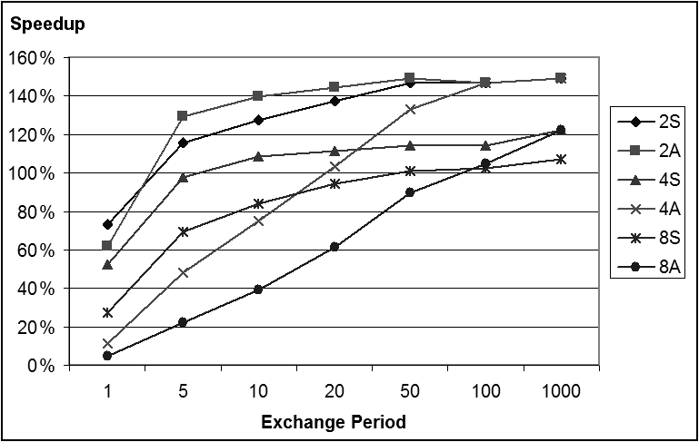Figure 2. Speedup for the Rosenbrock function as a function of the exchange period

Since the optimal solution has been found by the GA in many cases for this problem, as a measure of fitness we have used the percentage of runs in each case where the optimal solution was found. Figure 3 shows this parameter plotted as a function of the synchronization period, where we separated the plot by number of processes for a better visual understanding.

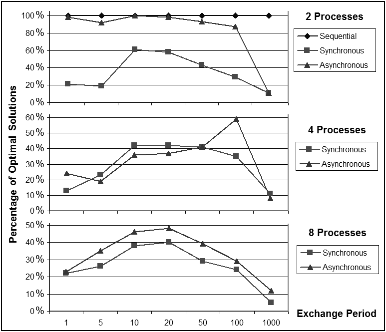Figure 3. Percentage of optimal solutions found as a function of the exchange period

This figure indicates that with 2 processes and a communication period of 10 or 20, the asynchronous model finds the optimal solution almost all of the 100 runs and can match the performance of the sequential model. For most of these runs, the asynchronous model performs better than the synchronous model. We can also note that for a higher number of processes, splitting each of the variables x and y themselves among the processes is not beneficial. This suggests that in general, the number of processes should not exceed the number of variables in the fitness function.

Overall, a synchronization period of 10 or 20 seems to be the best choice. This is consistent with results that were presented in[3,11].

The fitness itself is only half of the story. A remarkable thing about these experiments is that the number of generations that are necessary to achieve a given performance changes substantially from one setting to another. Thus, Figure 4 shows this measure as a function of the synchronization period. From this figure we can see that even though the algorithm doesn't find the optimal solution as frequently under the parallel models, the convergence is much faster in general. This suggests that for harder problems for which an optimal solution is not known, as for example, the motorcycle configuration problem, the parallel model is likely to achieve a reasonable fitness value faster.

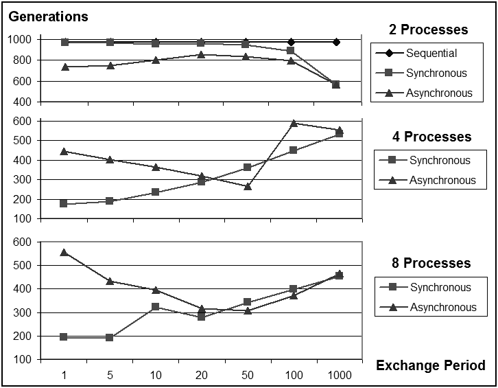Figure 4. The number of generations to achieve the fitness as a function of the exchange period

We have also performed some T-Tests comparing the fitness achieved under each parameter setting and a given value of the exchange period with the one achieved with the same parameter setting and the next value of the exchange period. Table 12 summarizes these results.

Table 12. T-Test for the significance of the fitness difference Exchange Period Significant Not Significant Sequential 1 2S, 4SA, 8SA 2A 1 5 All 5 10 All 10 20 2S 2A, 4SA, 8SA 20 50 2A, 4S, 8A 2S, 4A, 8S 50 100 2SA, 4A, 8S 4S, 8A 100 1000 All

5. Conclusions

In this paper we presented a shared memory parallel model of genetic algorithms designed to take advantage of multiple CPU cores in common current architectures. We have tested our model with three sets of problems of various difficulties on four different platforms with several types of processors and operating systems. Each problem presents different separability properties.

The experimental results presented in Section 4 explore the performance of the parallel model on several levels. First, in what concerns the speedup, for the benchmark functions there is a clear improvement on the platforms with multiple CPUs. A more modest but still noticeable speedup can be observed as well for the more difficult problem of configuring the autonomous pilot. The best speedup is around 185% on 2 CPU cores and around 223% on 4 CPU cores.

In terms of average fitness achieved in 1000 generations, for all test problems we can observe that the parallel model outperforms the sequential model for a number of processes less or equal to 4, which is also the maximum number of available cores on our test platforms. For the Rosenbrock function, the sequential model was able to find the optimal solution 100% of the time in 1000 generations, and this is also the case for the asynchronous model with 2 processes. For the deceptive problems, we see about 12% fitness improvement in the best case. For this problem, the parallel model was able to fine-tune the search to smaller parts of the chromosome and thus, improve the performance. For the motorcycle problem, we see an improvement of 3.5% in the best case.

A comparison of the synchronized and asynchronized schemes shows an improvement in speedup for the asynchronous model without loss in performance. Another set of experiments have shown that the synchronization and communication period of 10 generations that we have chosen is a nearly optimal choice of balancing between the speedup and fitness performance for both the synchronized and asynchronous models.

On the subject of problem separability, several conclusions can be drawn from our experiments. The speedup can be better improved for separable problems, which is to be expected. The fitness improvement is also more impressive for the more separable problems. A higher division of the chromosome is also more beneficial to problems that are more separable. With a division into 2 processes, though, an improvement can be observed for all the problems, even the non-separable ones. This means that even though our algorithm is more efficient for separable problems, it can still present some advantages even for non-separable ones.

In conclusion, our model presents a valid approach to taking advantage of the multi-core computing technologies that are now widely available, even for non-separable problems, and a strict synchronization between the processes is not a benefit in terms of performance.