D. Benazzouz , M. Amrani , S. Adjerid
Solid Mechanics and Systems Laboratory (LMSS), M’Hamed Bougara University, Boumerdes, UMBB Algeria
Correspondence to: D. Benazzouz , Solid Mechanics and Systems Laboratory (LMSS), M’Hamed Bougara University, Boumerdes, UMBB Algeria.
| Email: |  |
Copyright © 2012 Scientific & Academic Publishing. All Rights Reserved.
Abstract
This paper presents the retro-propagation algorithm for tuning the parameter of Artificial Neural Networks used by pharmachemical industry. The obtained numerical test results on lubrication and air circuits shown that the proposal improves the performance in terms of number of iterations and reliability of the models. BEKER Laboratories production line, is a Pharmaceutical production company located at Dar El Beida (Algiers-Algeria), was kept as the main target of this study. After careful inspection, the weakest and the strongest points of the system were identified and the most strategic equipment within the line (the compressor) was taken as the equipment of focus. From this specific point, failure simulations are most adequate and from this selected target, the designed system will be better positioned for failure detection during the production process. The efficiency of this approach is its fast learning, and its accuracy of detecting failure which is of the order of 10-3.
Keywords:
Artificial Neural Networks , Industrial Diagnosis , Industrial Monitoring, Gradient back, Propagation Algorithms
1. Introduction
Nowadays, the preventive maintenance domain has tendency to become an entire part in the market. The industrial systems became increasingly complex. For that, it is necessary to permanently supervise them in order to prevent any incident, to detect an eventual faulty in the equipment which allow a good quality of service. Emerging preventive maintenance domain tends to establish itself as the sole market, mostly due to the more complex growing industrial systems. Hence, permanent industrial supervision is becoming more and more vital to maintain competitive production qualities.Due to the ease of their implementation and their high reliability[1-3], the Artificial Neural Networks (ANNs) by their nature are most suited for extremely nonlinear processes. Hence, they are quiet often found within the industrial monitoring systems[5-6].Herein, we introduce an efficient neuronal approach, which was adapted to a pharmachemical industry from BEKER Laboratories. The main task was to determine and situate strong and weak points within the production line, based on the true data generated by the sensors; which are specific to the compressor. Notice that we want to recognizeif there is any failure and also what kind of failure the system has. We want to predict the system behavior while it is operating. Once done, this will make the automation of the diagnosis process doable[4]. The approach is based on the gradient back-propagation multilayer network because of it contains one or more hidden layers that can treat strongly nonlinear industrial systems, which we cannot treat with mathematical approach. Moreover, it is used for its fast learning and for its ability of generalization and classification.
2. Description of Beker Workshops Laboratory
BEKER Laboratories is a pharmaceutical drugs company, established in Algiers Algeria since 2005. The main composition structure of this company is as follows:Production Line UnitQuality Assurance LaboratoryResearch and Development LaboratoryWorkshop Unit.Our study was based on the production line structure as shown in Fig.1, as it had all the required elements that apply to the objective of this paper. Within this production line the air compressor constitutes the central unit that feeds all the other parts; therefore our focus was mainly oriented in the observation of this unit represented in Fig.1. A. Compressor Operating Principle and its ImportanceThe air compressor is a rotary two-stage type with lobes coupled with an electric motor[8]. The ambient air is condensed by the compressor in two stages; the air enters the low pressure zone to be cooled, then it enters the high pressure zone.The resulting air leaves the compressor with a desired pressure equal to 7 bars. This pressure will be distributed via piping towards all the machines as shown in Fig.1. The availability of the pressure air is synonym of the availability of the production. If there is any trouble in the pressure circuit no machine will be functioning. Therefore, the reliability of the compressor is also synonymous of the preventive maintenance quality. For these reasons, the supervision of the air compressor is the best strategy to maintain the production of the drugs to its optimum. 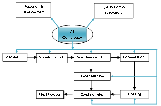 | Figure 1. Production Line of BEKER Laboratory |
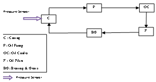 | Figure 2. Lubrication Circuit |
3. Air Compressor Model
The air compressor is composed of two main circuit modules; the lubrication circuit part, and the air circuit part. For the sake of simplicity the compressor is decomposed in two parts, denoted A and B.● Part A: Lubrication C ircuit, the compressor’s casing gear box holds a pressure sensor of type PT45 that takes measurements of the oil pressure. In fact, the oil pressure is a parameter used as an entry in the ANN as the indicator of faulty in this module. The oil pressure is specific to this compressor and varies between 1.5 and 2.7 bars; therefore any value out of this range is considered as a faulty of this module. The zones of good functioning are denoted by the symbol '1', and the zones of faulty are denoted by the symbol '-1'. These symbols are considered as the output of the ANN. Fig. 2 represents the lubrication circuit. The oil pressure is monitored in ordered to obtain a real time measurement of the lubrication module.● Part B: Air Circuit, in this part we have two pressure and three temperature sensors; which means that we do have two parameters to monitor. The pressure and the temperature readings are the most significant indicators of the breakdowns in the air circuit module. Fig.3 shows the air circuit and the positions of the sensors.The surveillability of this circuit will be based on monitoring all these parameters separately. Since each parameter is an entry to the ANN, we will have 5 neural networks that supervise all those parameters in parallel.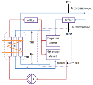 | Figure 3. Air Circuit |
4. Compressor Neuronal Model
The proposed neural model is based on the gradient multi-layer retro-propagation network '1-12-1', containing one layer entry with one neuron, one hidden layer with twelve neurons and one output layer with a single neuron. The optimization of the neural model is performed at random following these options:First, by varying the number of neurons within the hidden layer, then by comparing all various architectures. Based on this comparative study, which gives several training tests, we obtained this configuration of 12 neurons in the hidden layer. This gave a fast convergence and a good result with an error of around 10-3 during the training time. With this choice we were able to avoid the overtraining phenomena as well as the local minima. This overtraining (over-learning) is avoided in a stochastic manner (randomly, notice that the artificial intelligence method is stochastic method) i.e. the adequate parameters of the ANN are determined after various tests. Among the parameter that can be influenced during the test are: the neural number in the hidden layer, the initial values of weights and biais and the iteration number. Second, by stochastically initializing several times the weight values, we found that the weight values within an interval of[-0.5, 0.5] were better suited for our application.Third, we fixed the number of iteration to 1300 which is largely sufficient for this application.The training data are data given by the manufacturer and are listed in table1 which gives the specifications of the sensors functioning values ranges of the air compressor.| Table1. Sensor Functioning Values Ranges of the Air Compressor |
| | Compressor parameters | Min. Value | Ave. Value | Max. Value | | Lubrifiante Circuit | | PT45 oil pressure | 1.5 bars | 2 .5 bars | 2.7 bars | | Air Circuit | | PDT02 pressure, air filter (ΔP) | -0.100bar | -0.044bar | -0.044bar | | PT29 output air pressure | 4 bars | 7 bars | 7 .3 bars | | TT11 element output temperature (BP) | 100 °C | 220 °C | 225 °C | | TT18 input temperature (HP) | 60°C | 65°C | 75°C | | TT21 element output temperature (HP) | 100°C | 220°C | 225°C |
|
|
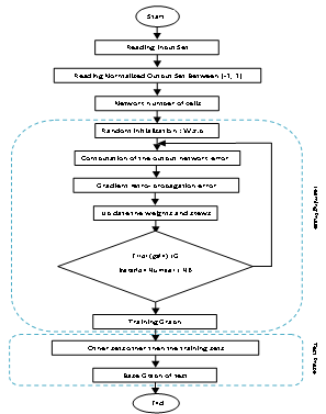
A.Training PrincipleThe back-propagation algorithm[7] is there to tune the parameters (weight and contour), until reaching the desired output values (these values are within the interval[-1, 1]). The convergence was obtained far enough to the fixed value of iteration.B.Training Parameters Choice a- The error (goal): It is the error targeted by the cost function. We have settled down for an error in the order of 10-3.b- The iteration number: it is the number for which the algorithm of retro-propagation is executed. It might be that the network converges before reaching the predetermined number of iterations. Or it might as well not converge at all.c- The training rate: the performance of the gradient retro-propagation algorithm is sensitive to the changes of the training rate. If this is very high, the algorithm can become unstable, and if it is too small, the algorithm may take a too much time to converge.d- Activation Function: we have used the activation function the sigmoid type bipolar, nonlinear and increasing, it allows us to introduce a threshold and a saturation to limit the amplitudes of the network outputs which are between[-1,1].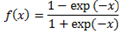 To implement the gradient retro-propagation training algorithm of the network, we apply the algorithm according to following stages:Step1: normalized input/output reading values Step2: set the cells numbers '1-12-1'. Step3: random initialization of the weight and skew values in the[- 0.5, 0.5] interval.Step4: iteration number (NB=1300), training gain (g=0.001).Step5: error calculation to be retro-propagated.Step6: modification (or adaptation) of the weights and skews and go to step4.step7: training results. In order to check the detection area of the good and faulty operation, we used various values in the training phase defined by the graphs 'test bases'. Fig. 4 and Fig. 5 represent respectively the neuronal model and the flow chart of the algorithm.
 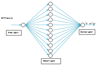 | Figure 4. Neural Model |
 | Figure 5. Algorithm Flow Chart |
5. Simulation and Results
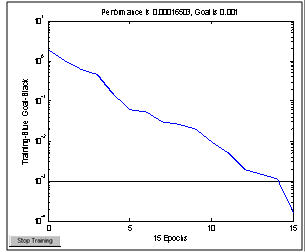
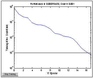
The program was developed under MATLAB 7.0. The obtained results of the lubrication circuit and the air circuit are as follows:●Part A: Lubrication Circuit A-Training We start with the network training simulation for the oil pressure lubrication circuit. The normal range of the oil pressure is[1.5, 2.7] bars, all other values out of this range cause an abnormal situation and leads to a faulty.Fig.6.1 shows that the convergence is reached around 240 iterations; this enabled us to say that the network (1-12-1) has performed a good training according to the desired objective.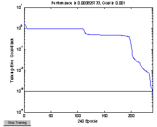 | Figure 6.1. Training Simulation Network |
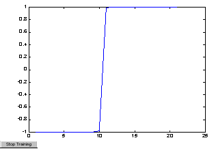
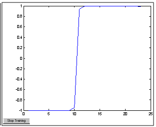
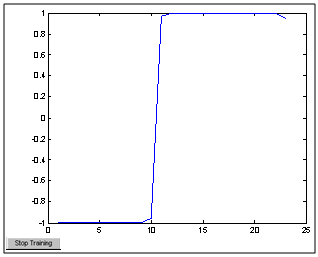
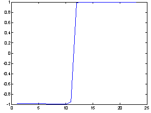 | Figure 6.2. Test Base |
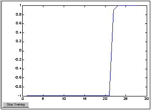
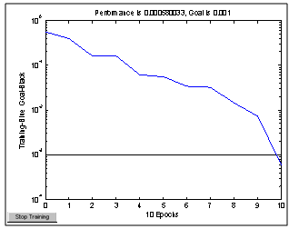
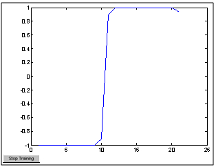
b- Simulation of good and faulty operation zones After the training it is useful to know if the network (1-12-1) is able to recognize faulty for other situations which are not known by ANN. We mean to recognize the good and faulty operation points, other than those which are given in the training phase. Fig. 6.2 shows a test base for other set of points other than used in the training phase. The values of the basic test graph are between[-1, 1] which reflects a desired output of the network.●Part B: Air Circuit In this part, we will supervise separately the parameters of the air circuit. We start with the training phase with some set of points than we try other set of values other than those given in the training and we will proceed with this manner for the rest of parameters to be supervised. The air pressure filter operation range is[-0.1, -0.044] bar. All values within this range are considered to be in normal operation otherwise we are in faulty operation. Fig. 6.1a shows the simulation of the network training which converges after 10 iterations only. Fig. 6.1b shows a test base. The test was carried out with other sets of entry. This shows that the network is reliable and able to detect the normal and the faulty operation. Thus the supervision real time is possible.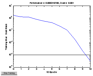 | Figure 6.1a. Training Simulation Network |
 | Figure 6.1b. Test Base |
¾Pressure Simulation, Output Air of the Compressor The operating range of the pressure at the output of the compressor is[4, 7.3] bars, Fig. 6.2a shows the simulation of the network training which converges after 20 iterations. Fig. 6.2b shows the test base of the output air of the compressor.¾Temperature Simulation, Output Low Pressure The operating range of the temperature at the output low pressure is[100, 225] °C. Fig. 6.3a shows the simulation of the network training (1-12-1) which converges after 15 iterations. Fig. 6.3b shows a test base of the output low pressure.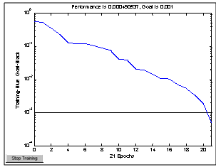 | Figure 6.2a. Training Simulation Network |
 | Figure 6.2b. Test Base |
 | Figure 6.3a. Training Simulation Network |
 | Figure 6.3b. Test Base |
 | Figure 6.4a. Simulation of Drive of the Network |
 | Figure 6.4b. Test Base |
 | Figure 6.5a. Training Simulation Network |
 | Figure 6.5b. Test Base |
¾Temperature Simulation, Input High PressureThe operating range of the input high pressure is[60, 75] °C. Fig. 6.4a shows the training simulation network (1-12-1) which converges after 10 iterations. Fig. 6.4b shows the test base of the temperature at high input pressure.¾Temperature Simulation, Output High PressureThe operating range of the output high pressure is[100, 225]°C. Fig. 6.5a show the training simulation network (1-12-1) which converges after 15 iterations. Fig. 6.5b shows a test base of the temperature at the output high pressure.
6. Conclusions
The used neural approach model of (1-12-1) network allows us to supervise in real time the pharmaceutical BEKER Laboratory line production. The training simulation sets of the network shows the following quality results:The fast convergence results was showed in the training graphs where some iterations were reached from 10 to 20 for the air circuit case and 240 iterations. The phenomena of on-training and local minima did not appear. This confirms a satisfactory choice of the parameters in the gradient retro-propagation algorithm. All the test bases show the desired outputs of the network[-1, 1], therefore the detection of the faulty is guaranty.It is not necessary to validate data or results with other methods of validation (k-fold), we are not in a theoretical or ideal case, our application is useful because we obtain valuable results and were verified by the feedback knowledge of the operators on site. From this, we can say that the network is able to detect any anomaly in the system by just controlling the output of the network. We can supervise any anomaly of the controlled parameters of the compressor. This facilitates the diagnosis of the machine and at the same time enhances the preventive maintenance more effectively. The weaknesses of the ANN approach are encountered while testing the network optimization. The ANN parameters are not fixed at the beginning; they are determined by testing (randomly).
References
| [1] | M.DJOUADA, ’Diagnostic des défauts par un couplage réseaux de neurones artificiels – algorithmes génétiques’, Laboratoire de Mécanique de Précision Appliquée. Université Farhat Abbas, Sétif, Algérie 19000. Novembre. |
| [2] | ‘Réseaux de Neurones’, M. Larizeau, Université de Laval, Canada, 2004. |
| [3] | N. Benahmed, ’Optimisation de réseau de neurones pour la reconnaissance de chiffres manuscrits isolés’, Thèse de doctorat, Université de Québec, Canada, 2002. |
| [4] | R. Casimir, ’Diagnostic des défauts des machines asynchrones par reconnaissance des formes’, Thèse de doctorat, Ecole Centrale de Lyon, France, 2003. |
| [5] | D. Maquin, ’Surveillance à base de modèle’, Ecole des journées doctorales d’Automatique–JDMACS, Reims Champagne, France, 11-12 juillet 2007. |
| [6] | D. Racoceau, ’Contribution à la surveillance des systèmes de production en utilisant les techniques de l’intelligence artificiels’, Thèse de doctorat, U. de Lilles, France, 2006. |
| [7] | F. Denis, R. Gilleron, P.J Boris, ’Définition et expressivité des réseaux multicouches L’algorithme de rétro-propagation du gradient’, 2 Nov. 2007. |
| [8] | Documentation technique du fabricant BEKER, Dar-El-Beida, Alger, Algérie, 2007. |
 Abstract
 Reference
 Full-Text PDF
 Full-Text HTML