1. Introduction

From journal study, it has been proved that the main application of principal component and factor analysis are (1) to reduce the number of variables and (2) to detect the structure in the relationship between variables, that is classify variables. Therefore, factor analysis and principal component analysis are applied as data reduction or structure detection methods. The term factor analysis was first introduced by Thrustone[6], 1931.A hands-on how-to approach can be found in Stevens(1986); more detailed technical descriptions are provided in Cooley and Lohnes (1971); Harman (1976);Kim and Muller (1978a,1978b); Lawley and Maxwell(1971) Lindeman, Merenda and Gold(1980); Morrison(1967);or Mulaik(1972). The interpretation of secondary factors in hierarchical factor analysis, as an alternative to traditional oblique rotational strategies, is explained in detail by Wherry (1984). When mining a dataset comprised of numerous variables, it is likely that subsets of variables are highly correlated with each other. Given high correlation between two or more variables it can be concluded that data that these variables are quietly redundant thus share the same driving principal in defining the outcome of the interest. The use of principal component analysis techniques [3] is well established in many fields such as pharmacology, climatology, numerous aspects of the life science, economics, ( Jolliffe, 1986,Faloutsos,Korn, Labrinidis, Kaplunuorich ,& Perkovic 1997;Preisendorfer, 1988; Shum,lkeuchi, & Reddy 1997) and even religious studies! See example Walker (2001) who has provided a very illustrative a and imaginative use of this statistical methodology.

S. F. Brown, A. Branford and W. Moran[33] proposed that artificial neural networks were powerful tool for analyzing data sets where there were complicated nonlinear interactions between the measured inputs and the quantity to be predicted. F. G. Donaldson and M. Kamstra[42] investigated the use of Artificial Neural Network (ANN) to combine time series forecasts of stock market volatility from USA, Canada, Japan and UK. The authors presented techniques of combining procedures to a particular class of nonlinear combining procedure based on Artificial Neural Network (ANN). H. J. Zimmermann[34] presented the application of fuzzy linear programming approaches to the linear vector maximum problem. It showed the solutions obtained by fuzzy linear programming were always efficient solutions. In a fuzzy environment a decision could be viewed as the fuzzy objective function, which was characterized by its membership functions and the constraints. G. A. Tagliarini, J. F. Christ and E. W. Page[36] demonstrated that artificial neural networks could achieve high computation rates by employing massive number of simple processing elements of high degree of connectivity between the elements. Neural networks with feedback connections provided a computing model capable of exploiting fine-grained parallelism to solve a rich class of optimization problems. This paper presented a systematic approach to design neural networks for optimization applications. M. Laviolette, J. W. Seaman Jr, J. D. Barrett and W. H. Woodall[35] presented that fuzzy set theory had primarily been associated with control theory and with the representation of uncertainty in applications in artificial intelligence. Fuzzy methods had been proposed as alternatives to statistical methods in statistical quality control, linear regression and forecasting. M. Laviolette, J. W. Seaman Jr, J. D. Barrett and W. H. Woodall[35] and stated the difference between fuzzy and probabilistic logic and stated advantages of fuzzy logic controller. The distinction between randomness and fuzziness was based on the different types of uncertainty captured by each concept. R. G. Alamond[37] presented the comparison between fuzzy set theory and probability theory, problems with probability, certain applications in fuzzy set theory. Uncertainty meant the incident, which was not known to happen in a single experiment but could be predicted the behavior of many similar experiments.

Melike Sah and Konstantin, Y.Degtiarev[28] proposed a novel improvement of forecasting approach based on using time-invariant fuzzy time series on historical enrollment of the university of Alabama. They compared the proposed method with existing fuzzy time series time-invariant model based on forecasting accuracy.

Tahseen Ahmed Jilani, syed Muhammad, Agil Burney and Cemal Ardil[38] proposed a method is based on frequency density based partitioning of the historical enrollment data. They proved that the proposed method is the based method of forecasting accuracy rate for forecasting enrollments than the existing methods.

Using the value of shoot length, it has been observed that artificial neural network gives better results as compared to fuzzy logic and statistical models[15]. An effort has been made using neural network based on fuzzy data on mango export quantity and revenue generated from it.[16].

The different type of research work ([19]-[27]) has been carried out using fuzzy logic and artificial neural network to forecasting rainfall, temperature and thunder strorms. They compared the proposed method with existing fuzzy time series time-invariant model based on forecasting accuracy. S.Kotsiantis, E. Koumanakos, D. Tzelepis and V. Tampakas[29] explored the effectiveness of machine learning techniques in detecting firms that issue fraudulent financial statements(FFS) and deals with the identification of factors associated to FFS. Tahseen Ahmed Jilani, Syed Muhammad, Agil Burney and Cemal Ardil[30] proposed a method is based on frequency density based partitioning of the historical enrollment data . They proved that the proposed method is the based method of forecasting accuracy rate for forecasting enrolments than the existing methods. A lots of research work also have been conducted for the prediction of several things ([19]-[30]).

In this paper, an effort has been made to find the significant environment parameters which are affected the growth of mustard plant using principal component and factor analysis. The environmental parameters like maximum and minimum temperature, rain fall; maximum and minimum humidity, soil moisture at different depth and sun shine have been taken. Finally, the parameters have been reduced and only few parameters have been used to predict the growth of mustard plant. To predict the growth of the mustard plant can be measured by observing the growth of its shoot length only. As new leaves of plant may appear and old leave may fall down. The roots are going deeper to deeper inside the soil. This is the reason, the shoot length has been considered here to predict the productivity of mustard plant. At initial stage, using the reduced parameters, the shoot length of the mustard plant has been predicted by artificial neural network (ANN) . Least square method has been applied on predicted shoot length to find the shoot length at maturity. Finally, the productivity of plant has been predicted from shoot lengthy at maturity (after 95 days).This type of effort has not been used in prediction the growth of mustard plant that is the reason for ma king the effort in this paper.

2. Theoretical Illustration of Principal Component and Factor Analysis and ANN

2.1. Principal Component Analysis

PCA ([1]–[5]) transforms the original set of variables into a smaller set of linear combination that account for most of the variance of the original set. The principal component analysis has been determined almost total variation of the data as much as possible using few factors [43]. The first principal component, PC_(1), accounts the maximum of total variation in the data. PC(1) is represented by linear combination of the observed variables Xj, j=1,2,3….p – say

PC ₍₁₎ = w₍₁₎₁X1 +w₍₁₎₂X2+……+w_(1)pXp ,where the weights w(1)1, w(1)2, ….. w(1)p have been chosen to maximize the ratio of the variance of PC(1) to the total variation, subject to the constraint that S 1-p w²₍₁₎=1

Now, The second component, PC(2), is uncorrelated with PC(1) and represents the maximum amount from the total variation not already accounted for by PC₍₁₎. In general, the m^th principal component is that weighted linear combination of the X ‘s

PC(m) = w_(m)1X1 +w_(m)2X2+……+w_(m)pXp,which has the largest variance of all linear combinations that are uncorrelated with all of the previously extracted principal components. In this way, as many as possible principal components are extracted.

2.2. Factor Analysis

Factor analysis is used to identify underlying variables, or factors which are correlated within a set of observed variables [6]. Factor analysis has also been used in data reduction by identifying a small number of factors of the variance observed in a much larger number of variables.

Assume that our X variables are related to a number of functions operating regularly. That is,

X₁=α₁₁F₁+ α₁₂F₂+ α₁₃F₃+ . . . . + α_1mF_m

X₂=α₂₁F₁+ α₂₂F₂+ α₂₃F₃+ . . . . + α_2mF_m

X₃=α₃₁F₁+ α₃₂F₂+ α₃₃F₃+ . . . . + α_3mF_m

(1)

Where X’s a variables with known data, α a constant and F a function, f( ) of some unknown variables. The loadings emerging from a factor analysis are constants. The factors are the F functions. The size of each loading for each factor measures how much that specific function is related to X. For any of the X variables of equation 1 may be writing

(2)

With the F’s representing factors and α’s representing loading.

2.3. Artificial Neural Network (ANN)

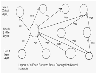
An ANN (Artificial Neural Network) is composed of collection of interconnected neurons that are often grouped in layers. In feed forward back propagation neural network (FFBP NN) does not have feedback connections, but errors are back propagated during training. Errors in the output determine measures of hidden layer output errors, which are used as a basis for adjustment of connection weights between the input and hidden layers. Adjusting the two sets of weights between the pairs of layers and recalculating the outputs is an iterative process that is carried on until the errors fall below a tolerance level. Learning rate parameters scale the adjustments to weights. A momentum parameter can be used in scaling the adjustments from a previous iteration and adding to the adjustments in the current iteration. The layout of feed forward back propagation neural network is furnished in figure 3.

Figure 3.

Table 1(a). Data related Environmental parameter MaxiTemp. MinTemp. RainFall Max.Humidity MinHumidity D1 D2 D2 SunShine 27.4 15.6 28.8 95.75 58.35 16.9 21.96 28.13 7.77 25.9 14.15 19.2 96.68 59.48 14.83 19.63 26.1 8.11 24.4 12.7 9.6 97.6 60.6 13.23 17.7 23.76 8.32 24 12.33 29.68 97.78 60.73 11.86 16.33 21.63 7.44 23.6 11.95 49.75 97.95 60.85 18.86 14.9 19.76 7.18 23.2 11.58 69.83 98.13 60.98 11.03 15.03 19.3 7.62 22.8 11.2 89.9 98.3 61.1 10.76 14.93 19.13 8.48 24.08 12.38 74.73 97.93 59 10.8 14.83 18.96 7.32 25.35 13.55 64.55 97.55 56.9 9.8 13.8 17.96 7.14 26.63 14.73 51.88 97.18 54.8 9.3 13.1 17.03 6.05 27.9 15.9 39.2 96.8 52.7 8.13 12.36 16.03 7.48 28.53 16.38 79.3 96.43 51.83 7.86 11.86 15.46 9.42 29.15 16.85 119.4 96.05 50.95 6.96 10.13 14.33 7.22

Table 1(b). Initial Shoot Length of different time Instances Time Instances Shoot Length 1 19.00 2 22.00 3 24.00 4 27.00 5 31.00 6 33.00 7 34.00 8 36.00 9 38.00 10 42.00 11 46.00 12 50.00 13 54.00

Table 1(c). Shoot length and Pod Yields at maturity After 95 days) Shoot Length(Height) Pod yield(gm) 122.6 3.991 135.5 2.679 140.8 7.281 141.8 7.47 144.6 7.401 146 7.5 149.5 7.64

3. Data used in this Paper

A statistical survey has been conducted by a group of certain agricultural scientists on different mustard plants under the supervision of Prof. Dilip De, Bidhan Chandra Krishi Viswavidyalaya West Bengal, India. The objective of the survey was to find the productivity of different mustard plant at maturity (after 95 days).The data has been collected in two stages. At first, after plantation, the reading has been taken on different parameters like shoot length, number of leaf, number of roots and root length of the plant up to 28 days. The data has been taken in some day’s interval so that the changes of parameters have been identified. Secondly, the shoot length and productivity (seed weight) at maturity (after 95 days) have been taken. The environment data like maximum and minimum temperature, rain fall; maximum and minimum humidity, soil moisture at different depth and sun shine have been collected during the year. In another paper [39], the authors have proved that the mustard plant must be planted from November to February. Now, except the shoot length, all other plant parameters cannot be measured as plant is growing. The leaves may appear and fall down and the roots are going inside the soil. So, shoot length has been used to predict the growth of mustard plant. In this paper, environmental data during initial growth(November to February) , initial shoot length of different time instances and seed weight at maturity from this survey are furnished in table 1(a), 1(b) and 1(c).

4. Method

4.1 Principal Component Analysis

Step 1: After the plantation, the environmental parameters have been collected during the harvest period of growing stage of mustard plant is furnished table 1(a). Using Statistica 7 software package, the correlation matrix[40] of table 1(a) is furnished in table 2.

Step 2: The eigen values, total variances, commulative eigen vector and percentage of contribution is furnished table 3.

Table 2. Correlation Matrix Variable Correlation Matrix Maxi Temp. Min Temp Rain Fall Max Humidity Min Humidity D1 D2 D3 Sun Shine Maxi Temp. 1.000 0.999 0.178 -0.917 -0.911 -0.425 -0.303 -0.279 0.039 Min Temp 0.999 1.000 0.146 -0.927 -0.897 -0.400 -0.269 -0.246 0.038 Rain Fall 0.178 0.146 1.000 0.0094 -0.434 -0.581 -0.719 -0.731 -0.007 Max Humidity -0.917 -0.927 0.009 1.000 0.678 0.110 -0.070 -0.098 -0.114 Min Humidity -0.911 -0.897 -0.434 0.678 1.000 0.690 0.656 0.643 0.039 D1 -0.425 -0.400 -0.581 0.110 0.690 1.000 0.772 0.779 -0.002 D2 -0.303 -0.269 -0.719 -0.070 0.656 0.772 1.000 0.993 0.164 D3 -0.279 -0.246 -0.731 -0.098 0.643 0.779 0.993 1.000 0.164 Sun Shine 0.039 0.038 -0.007 -0.114 0.039 -0.002 0.164 0.164 1.000

Table 3. The eigen values computed from table 2 Component Eigen values % Total variance Commutative Eigen value Commulative % 1 4.742622 52.69580 4.742622 52.6958 2 2.576152 28.62391 7.318774 81.3197 3 1.002231 11.13590 8.321005 92.4556 4 0.429760 4.77511 8.750766 97.2307 5 0.236331 2.62590 8.987097 99.8566 6 0.010602 0.11780 8.997699 99.9744 7 0.002276 0.02529 8.999975 99.9997 8 0.000021 0.00023 8.999996 100.0000 9 0.000004 0.00005 9.000000 100.0000

Step 3: When analyzing correlation matrices(table 2), the sum of the eigenvalues is equal to the number of (active) variables from which the factors were extracted (computed), and the "average expected" eigenvalue is equal to 1.0. Many criteria are used in practice for selecting the appropriate number of factors for interpretation; the simplest is to use (retain for interpretation) as many factors as the number of eigenvalues that are greater than 1. In this example, only the first three eigenvalues are greater than 1, accounting for approximately 92% of total variation. The values of all eigen values has been shown in figure 2.

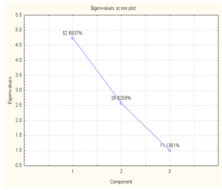Figure 2. Eigen Values

Table 4. Principal Component Analysis Eigenvalues, Number of components is 3 and Principal Component Analysis sum of variance 9.0000 Component Eigenvalues % Total variance Commulative Eigenvalue Commulative % 1 4.742433 52.69370 4.742433 52.69370 2 2.576318 28.62576 7.318751 81.31946 3 1.002246 11.13607 8.320998 92.45553

The eigenvalues in the table 4 are arranged in decreasing order, indicating the importance of the respective factors in explaining the variation of the data. The factor corresponding to the largest eigenvalue (4.742433) accounts for approximately 52.7% of the total variance. The second factor corresponding to the second eigenvalue (2.576318) accounts for approximately 28.7% of the total variance, and so on.

Step 4: Another method for determining the number of factors to interpret (retain) is to construct the so-called scree plot (Cattell, 1966). Specifically, the successive eigenvalues will be shown in a simple line plot is shown in Figure 1. Cattell suggests finding the place where the smooth decrease of eigenvalues appears to level off to the right of the plot. No more than the number of factors to the left of this point should be extracted.

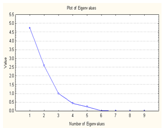Figure 1. Number of Eigen Values

Step 5: The eigen vector corresponding the table 1(a) has been furnished in table 5. The number of component components has been display corresponding the eigen value i.e three components (1, 2 & 3).

Table 5. Eigen Vector Variable Eigenvector and number of components are 9 Comp1. Comp2. Comp3. Comp4. Comp5. Comp6. Comp7. Comp8. Comp9. Maxi Temp. 0.376844 0.351089 -0.049277 0.004788 -0.060887 0.045167 0.109832 0.842154 0.072348 Min Temp 0.367258 0.368866 -0.057148 0.012133 -0.050944 -0.099814 -0.032073 -0.380394 0.753228 Rain Fall 0.278404 -0.335760 0.186305 -0.827185 0.250654 -0.092859 0.100982 0.034040 0.082540 Max Humidity -0.255216 -0.504113 0.020553 0.246988 -0.094492 -0.431998 0.400558 0.249690 0.448336 Min Humidity -0.447332 -0.114271 0.047172 -0.107519 0.137673 0.540210 -0.427212 0.247767 0.467255 D1 -0.362725 0.228962 -0.134402 -0.457405 -0.759098 -0.099693 0.053440 0.004963 0.002213 D2 -0.354890 0.373221 0.023754 -0.108974 0.405385 -0.651203 -0.346250 0.116450 -0.020937 D3 -0.349858 0.387868 0.016830 -0.104592 0.360005 0.258640 0.714849 -0.087072 0.028736 Sun Shine -0.021059 0.136358 0.968523 0.104869 -0.181156 -0.005230 0.000064 -0.004166 0.000298

Step 6: As the value of three eigen value has been calculated greater than 1.00. So, three components from table 5 have been taken and furnished in table 6.

Table 6. Eigenvector computed from table1(a) Variable Eigenvector and Number of components is 3 Variable Number Component1 Component2 Component3 Maxi Temp. 1 0.376844 0.351089 -0.049277 Min Temp 2 0.367258 0.368866 -0.057148 Rain Fall 3 0.278404 -0.335760 0.186305 Max Humidity 4 -0.255216 -0.504113 0.020553 Min Humidity 5 -0.447332 -0.114271 0.047172 D1 6 -0.362725 0.228962 -0.134402 D2 7 -0.354890 0.373221 0.023754 D3 8 -0.349858 0.387868 0.016830 Sun Shine 9 -0.021059 0.136358 0.968523

Step 7: To find the significant variable from table 6, the following method has been applied. In principal component analysis, one component is linear combination of all variables. To find the particular variable on which the components is mostly depend on, the following method has been described below

The first component corresponding to the first eigen value 4.742433 is most correlated with Min humidity (high negative correlation). So, component1 is dependent on min humidity. The other dependency can be found those variable which is under 10% of min humidity (highest value in component 1) i.e., (-0.447332—0.0447332) or –0.4025988. From the component1 (table 6), it has been observed that the value of others variables less than 0.4025988 (negative correlation).

So, no other variable is play dominant role in component 1. If, more than one variable have been predicted as significant variables, one correlation matrix will be computed and depending on correlation, the significant variable will be calculated.

Thus in component 2 corresponding eigen value 2.576318 and it’s dominating variable max humidity and after reduction of 10% of this is 0.4537017 not correlated with other variables.

Finally, from component 3 sun shine is most dominant variables.

Step 8: It has been observed that component1, component2 and component3 are dependent three variables min humidity, max humidity and sun shine. So, without considering 9 variables, three has been given 92% solution of this problem.

4.2. Factor Analysis

Step 1: The same data furnished table 1(a) has been used in factor analysis and Using Statistica 7 software package, factor loading have been calculated in factor analysis are furnished in table 7and table 8 The eigen values have been taken which are greater than 1. The factors have been taken same as number of eigen values.

Step 2: In factor analysis[41], one variable is linear combination of all factors. The factor value which is greatest of all factors has been mark in the row of all variables. In each factor, it has been found the greatest value from all marks values; the corresponding variable has been taken. Using this method, the variable Min humidity has been selected in factor 1 from table 8. From the other two factors, the height loading of other two factors are -0.805376 and 0.969639, i.e., max humidity and Sun Shine.

So, three variables max humidity, min humidity and sun shine have been calculated as the significant variables.

Table 7. Eigenvalues Value Eigen values % Total variance Cumulative Eigenvalue Cumulative % 1 4.742622 52.69580 4.742622 52.69580 2 2.576152 28.62391 7.318774 81.31971 3 1.002231 11.13590 8.321005 92.45562

Table 8. Factor Loadings (Unrotated) Variable Factor Loadings (Unrotated) (PCAapplication)Extraction: Principal components(Marked loadings are >.700000) Factor1 Factor2 Factor3 Maxi Temp. -0.827782 0.558140 -0.048038 Min Temp -0.807268 0.586862 -0.055871 Rain Fall -0.599427 -0.544217 0.188404 Max Humidity 0.566025 -0.805376 0.017682 Min Humidity 0.976464 -0.176991 0.047259 D1 0.785226 0.373728 -0.132438 D2 0.765244 0.604171 0.025844 D3 0.753988 0.627647 0.018927 Sun Shine 0.043168 0.213214 0.969636

4.3. Artificial Neural Network (ANN)

Under artificial neural network system, a feed forward back propagation neural network is used which contain three layers. One input layer, one hidden layers contain 3 neurons and one output layer contain one neuron.

The values of the artificial neural network parameters are initialized by newff function which has been created develop new neural network and initial values in matlab 7 package. The momentum parameter is taken as 0.7, learning rate 0.05, initial bias of hidden layer[0.2, 0.3, and 0.5] and initial bias of output layer is[0.2].

After applying PCA and Factor Analysis, the significant environmental parameters and related shoot length are furnished in table 9.

Table 9. Shoot length and significant environmental parameters Max Humidity Min Humidity Sun Shine Shoot Length 95.75 58.35 7.77 19.00 95.98 58.63 7.86 22.00 96.22 58.92 7.94 24.00 96.45 59.20 8.03 27.00 96.68 59.48 8.11 31.00 96.91 59.76 8.16 33.00 97.14 60.04 8.22 34.00 97.37 60.32 8.27 36.00 97.60 60.60 8.32 38.00 97.65 60.63 8.10 42.00 97.69 60.67 7.88 46.00 97.74 60.70 7.66 50.00 97.78 60.73 7.44 54.00

In neural network the input parameters are maximum humidity and min humidity and sunshine and target is shoot length. Using training and testing the predicted shoot length is furnished in table 10.

Table 10. Predicted Shoot Length using ANN Max Humidity Min Humidity Sun Shine Shoot Length Predicted Shoot Length 95.75 58.35 7.77 19.00 19.00 95.98 58.63 7.86 22.00 21.543 96.22 58.92 7.94 24.00 23.698 96.45 59.20 8.03 27.00 27.65 96.68 59.48 8.11 31.00 30.523 96.91 59.76 8.16 33.00 32.834 97.14 60.04 8.22 34.00 34.876 97.37 60.32 8.27 36.00 35.116 97.60 60.60 8.32 38.00 37.757 97.65 60.63 8.10 42.00 41.998 97.69 60.67 7.88 46.00 45.115 97.74 60.70 7.66 50.00 49.121 97.78 60.73 7.44 54.00 55.112

5. Result

In this methodology, it has been proved that out of nine environmental parameters, three of them (max humidity, min humidity and sun shine) have been are played significant role for growing the mustard plant. If these three parameters are available sufficiently, the growth of mustard plant will be healthy and they will be produced huge yields. The shoot length can be predicted using ANN which furnished table 7 and linear equations. The final shoot length after 95 days is 135.88 cm and the corresponding pod yield has been predicted 2.679gm (from table 1(c)).

6. Conclusions and Future Work

The principal component and factor analysis, same result can be produce using fewer parameters without considering all related parameters for a physical problem. The ANN used for training and testing to predict the productivity after finding the shoot length at maturity. It is a supervise learning which provide the target. This result can be cross examined using fuzzy logic, genetic algorithms in future.

ACKNOWLEDGMENTS

The authors would like to thank to the All India Council for Technical Education (F.No-1-51/RID/CA/28/2009-10) for funding this research work.