1. Introduction

In recent decades, artificial neural networks (ANNs) have been extensively used in numerous applications. One of the important applications of ANNs is finding patterns or tendencies in data. ANNs are well suited for prediction and forecasting requirements such as: sale forecasting, industrial process control, oil and gas industry[1-3], hand-written word recognition, target marketing, pharmaceutical industry[4], etc. In this paper, we use ANNs to identify an industrial process. One problem with ANNs is their instability. It means that small changes in the training data used to construct the model may result in a very dissimilar model[4]. Also due to the high variance of SNNs, the model may exhibit quite a different accuracy facing unseen data (validation stage)[4]. Furthermore, in numerous cases, a SNN lacks precision. Breiman[5] has shown that for unstable predictors, combining the outputs of a number of models will reduce variance and give more precise predictions.

However, it is required that the individual neural networks in aggregation should be dissimilar and there is no advantage in aggregation of the networks if they are all identical[4]. The purpose of this paper is to identify an industrial plant. Because of the stated reasons, we will use MNNs or ensemble neural networks for identification. Thereare several different ensemble techniques, but the

This paper consists of the following: in sections 1 and 2 a detailed study of bagging and boosting is presented. In section 3 the desired industrial process is introduced and then the bagging and boosting algorithms for identification are applied to this process. Some results and conclusions are presented in sections 4 and 5. Finally, references are given in section 6.

2. Bagging

Bagging (an abbreviation of bootstrap aggregation) is one of the most extensively used ANN ensemble methods. The main idea in bagged neural networks is to generate a different base model instance for each bootstrap sample, and the final outputs are the average of all base model outputs for a given input[19-21]. Some of the advantages of bagging algorithm are as follows:

• Bagging reduces variance or model inconsistency over diverse data sets from a given distribution, without increasing bias, which results in a reduced overall generalization error and enhanced stability.

• The other benefit of using bagging is related to the model selection. Since bagging transforms a group of over-fitted neural networks into a better-than perfectly-fitted network, the tedious time consuming model selection is no longer required. This could even offset the computational overhead needed in bagging that involves training many neural networks.

• Bagging is very robust to noise.

• Parallel execution: although the boosting algorithm (discussed in the next section) has better generalization ability than the bagging algorithm, the bagging algorithm has the benefit of training ensembles independently, hence in parallel.

Presume the training dataset T is composed of N instances, where x and y are input and output variables, respectively. It is required to acquire B bootstrap datasets. As a first step, each instance in T is assigned a probability of 1/N, and the training set for each of the bootstrap member TB is created by sampling with replacement N times from the original dataset T using the above probabilities. Hence, each bootstrap dataset TB may have many instances in T repeated a number of times, while other instances may be omitted. Individual neural network models are then trained on each of TB. Therefore, for any given input vector, the bootstrap algorithm offers B different outputs. The bagging estimate is then computed by determining the mean of B model predictions (see Figure 1).

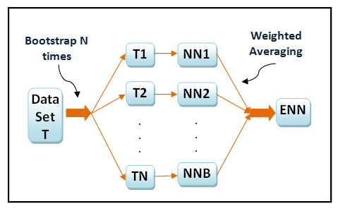Figure 1. Bagging neural network

The bagging algorithm can be summarized as:

1) Let B be the ultimate number of predictors required (obtained by trial and error).

2) Take a training set

3) For i = 1 to B do:

3.1) Make a new training set TB by sampling N items evenly at random with replacement from the data set T.

3.2) Train an estimator with the set TB and add it to the ensemble.

4) For any new testing pattern, the bagged ensemble output is given by the equation:

(1)

3. Boosting

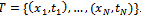
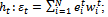
Contrary to bagging, boosting dynamically tries to generate complementary learners by training the next learner on the inaccuracies of the learner in the preceding iteration. At each iteration of the algorithm the sampling distribution depends upon the performance of the learner in the preceding iteration[22]. In spite of bagging algorithm which operates in parallel,boosting algorithm is executed sequentially. In boosting, instead of a random sample of the training data, a weighted sample is used to emphasis learning on the most difficult examples.

There are numerous different versions of the boosting algorithm in the literature. The original boosting approach is boosting by filtering and is explained by Schapire[23]. It requires a large number of training data, which is not practicable in many cases. This restriction can be overcome by using another boosting algorithm known as the AdaBoost[10]. Initially the boosting algorithm was developed for binary classification problems. Then boosting algorithmssuch as AdaBoosl.M1 and AdaBoost.M2[22] were developed for multi-class cases. In order to solve regression problems, Freund and Schapire[24]extended AdaBoost.M2 and called it AdaBoost.R. It solves regression problems by converting them to classification ones.

In this paper, we use AdaBoost.R2 for identification. This method is a modification ofAdaBoost.R and is described in[25,26]. A description of this algorithm (shown in Figure 2) is as follows: given that the training dataset T consists of N instances, where x and y are input and output variables, respectively. Initially each value in the dataset is allocated the same probability value so that each instance in the initial dataset has an equal likelihood of being sampled in the first training set; that is, sampling distribution, at step is equal to over all i, where to N.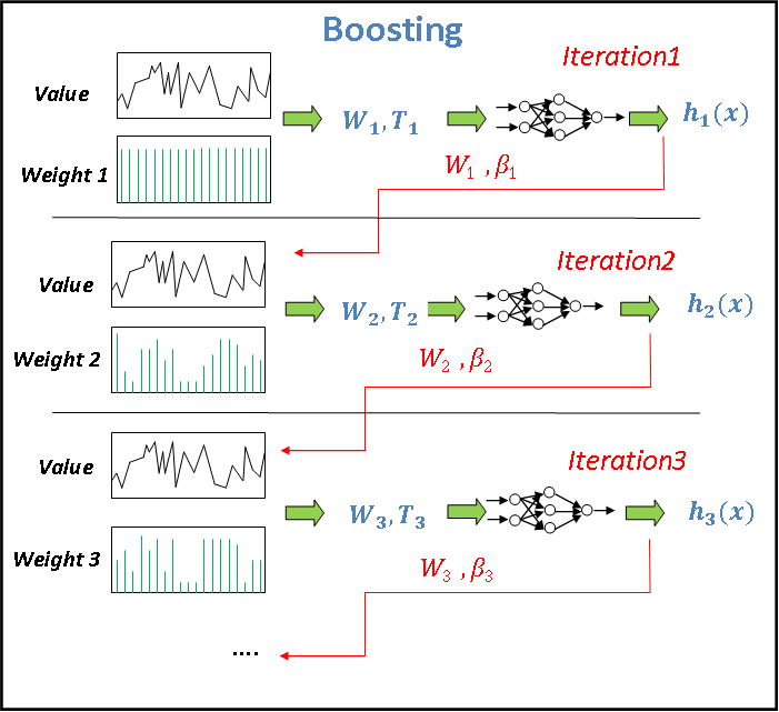

Figure 2. Boosting neural network

The boosting algorithm can be summarized as:

1) Input the labelled target data set T of theextent N, the maximum number of the iteration B, and a base algorithm learner. Unless otherwise stated, set the initial weight vector such that for .

2) For : (B can be determined by a trial and error method).

2.1) Fill the new training set with the distribution w^tand obtain a hypothesis

2.2) Compute the adjusted error for each instance:

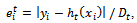(2)

(3)

2.3) Compute the adjusted error ofif, stop and set

2.4) Let

2.5) Bring up to date the weight vector according to the equation:

(4)

(z_tis a normalizing constant).

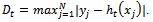
3) Output the hypothesis: = the weighted median of for, using as the weight for the hypothesish_t.

4. Process Modelling Using Bagging and Boosting

In this section, the bagging and boosting (Adaboost.R2) algorithms are used to identify a CSTR. Since, this paper is aimed at a black box model of the process, we need to collect data directly from the process or generate it by using simulation. For this purpose, data is taken from the Daisy website[27] which is an identification database.

The process is a CSTR where the reaction is exothermic and the concentration is controlled by adjusting the coolant. The input variable is the coolant flow rate (lit/min) and the output variable is the product concentration (mol/lit). Sampling time is 0.1 minutes and the number of samples is 7500. This data is in the form of a (3 × 7500) matrix. The first column of this matrix consists of time-steps, the second and third columns are input (coolant flow rate) and output (concentration) variables, respectively[27]. The input and output variables are shown in Figures 3 and 4. As shown in Figure 3, the input is constantly changing. So, the system is operated in dynamic mode.

In this paper, the bootstrap method is used to form subsystems in the bagging algorithm. The bootstrap procedure involves choosing random samples with replacement from a data set and analysing each sample the same way.

For the bagging algorithm, we use ten independent networks (B=10) and weights of each network are initiated randomly. Each network is composed of one hidden layer and the activation function of output layer is linear (purelin). However, the number of hidden neurons, their activation functions and learning algorithms are different. These specifications are listed in Table 1. For the hidden layer hyperbolic tangent sigmoid (tansig) and log sigmod (logsig) transfer functions are employed. For thenetwork training, Levenberg-Marquardt backpropagation (trainlm) and Beysian regulation backpropagation (trainbr) are used. Each individual network is trained for 10 iterations.

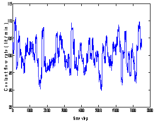Figure 3. Input variable (coolant flow rate)

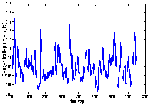Figure 4. Output variable (concentration)

As mentioned before, the system is in dynamic mode, so the previous inputs and outputs affect the output in the present time. In this case, the inputs to the network are the inputs in the present time the previous input and the previous output. So, the neural network consists of three inputs 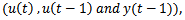and one output.

To determine the final predicted output of the trained ensemble, an average is taken over the predictions from individual networks.The results and conclusions are given in the following sections.

For system identification using the Adaboost.R2 algorithm, the number of iterations B should be determined. We select B to be equal to 20. All sequential networks are trained using the Levenberg-Marquardtback-propagationalgorithm. Each network consists of two layers. Activation functions in the output layer are “purelin” and in the hidden layer are “tansig”or “logsig”. The stopping goal for the single and every individual network is the mean squared error (mse = 0.000001). As described in the previous section, the lag space is equal to one; therefore, the number of sampled data points employed for modelling is 7499. So, the input-output data points are in the form of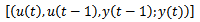. At the first iteration, all of the data points have equal chance to be selected. So, the probability of each data point to be elected is equal to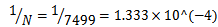. Using the Adaboost.R2 algorithm described in the previous section, we will see that the value of prior to the final iteration is less than the threshold value of 0.5, however at the final iteration . Hence, at this point the algorithm stops.

Tabe 1. Specifications of the networks used in this work network Number ofneurons Activation function in HL Training algorithm 1 5 tansig trainlm 2 6 tansig trainbr 3 5 logsig trainlm 4 6 logsig trainbr 5 5 tansig trainlm 6 6 tansig trainbr 7 5 logsig trainlm 8 6 logsig trainbr 9 5 tansig trainlm 10 6 tansig trainbr

5. Results

Table 2. Performance measures of the SNNs and MNN (thebagging neural network) Individual network Standard Deviation Sum Absolute Errors R-Squared 1 0.000747 0.320194 0.99855 2 0.000817 0.333045 0.99829 3 0.000850 0.509012 0.99837 4 0.000806 0.354326 0.99849 5 0.000767 0.364739 0.99858 6 0.000996 0.430697 0.99791 7 0.000800 0.330078 0.99839 8 0.000794 0.410069 0.99859 9 0.000915 0.413668 0.99790 10 0.000923 0.404273 0.99783 SNN 0.001040 0.411622 0.99732 MNN 0.000783 0.387010 0.99853

Table 3. Comparison between single neural network and multiple neural networks (theboosting neural network) Iteration Standard Deviation Sum Absolute Errors R-Squared Epsilon 1 0.000929 5.154209 0.99846 0.100205 2 0.000732 3.130475 0.00857 0.084706 3 0.000806 3.463874 0.99825 0.149771 4 0.000926 4.784363 0.99773 0.117025 5 0.001108 4.464097 0.99670 0.041901 6 0.000953 5.117671 0.99763 0.223891 7 0.001034 6.263647 0.99723 0.247154 8 0.001025 6.281662 0.99732 0.305718 9 0.001224 7.318611 0.99650 0.412131 10 0.001069 6.890501 0.99713 0.428246 11 - - - 0.7356287 SNN 0.000929 5.154209 0.99846 - MNN 0.000597 3.696289 0.99841 -

1) The performance measuresof the SNN (the complete data set is used to train the SNN) and ten individual neural networks used to construct the bagged neural network and the final MNN are shown in Table 2. As shown in this table, the accuracy of the MNN is comparable to the accuracy of the SNN. However, the variance of error in the MNN, compared to the SNN, has been significantly reduced. So, we can conclude that the bagging algorithm is successful in reducing the variance of error. In addition, thevalues tabulated for the square of the correlation coefficients(R-Squared) indicate that the regression in the MNN is better than the SNN.

2) The performance measures of the SNN and eleven sequential neural networks for constructing the boosted neural network or the final MNN are shown in Table 3. Using the Adaboost.R2 algorithm, we see that the value of prior to the eleventh iteration is less than the threshold value of 0.5, however at the eleventh iteration Hence, at this point the algorithm stops. Details of all the steps and the final results are shown in this table. The second column of the table shows that using the boosting algorithm leads to reductions of both of the error variance and modeling error in the MNN when compared against the SNN. It is clear from this table that regression of the MNN is better than the SNN (R-Squared closer to 1).

6. Conclusions

In this paper, identification of an industrial plant (CSTR) was performed using the SNN and MNN techniques. Industrial processes can be very complex and may have highly nonlinear properties. Hence, a single neural network cannot identify industrial processes with sufficient accuracy. We used multiple neural networks instead of a single neural network. We performed modelling by employing the bagging and boosting algorithms. As shown in this work, the MNNs generated by these two algorithms outperformed the performance of the single neural network. When bagging is employed, the accuracy of the MNN is comparable to the accuracy of the SNN. However, the variance of error in the MNN, compared to the SNN, has been significantly reduced. The boosting algorithm leads to the reductions of both of the error variance and bias of the MNN when compared against the SNN.Although the boosting algorithm ensures better generalization capability than the bagging algorithm, the latter algorithm has the benefit of training the ensembles individualistically, hence in parallel.