Jeremiah Anthony Samy 1, Prajindra Sankar Krishnan 1, Tiong Sieh Kiong 2
1Department of Electronics and Communications Engineering, Universtiti Tenaga Nasional, Kajang, 43009, Malaysia
2Power Engineering Centre / Department of Electronics and Communication Engineering, Universtiti Tenaga Nasional, Kajang, 43009, Malaysia
Correspondence to: Jeremiah Anthony Samy , Department of Electronics and Communications Engineering, Universtiti Tenaga Nasional, Kajang, 43009, Malaysia.
| Email: |  |
Copyright © 2012 Scientific & Academic Publishing. All Rights Reserved.
Abstract
Pattern recognition has been around for many years in the world of computer engineering and science. It’s a technique of learning and matching pattern data sets through memorization. There are two main techniques being used typically by most models which are the back propagation and feed-forward network from ANN (Artificial Neural Network). Both are used simultaneously in completing a task given. Discussed together in this paper are also the features of CLONALNet which is a part of AIS (Artificial Immune System). CLONALNet is a technique derived from the clonal se- lection family where it is a hybrid design of CLONALG and opt-AINet used for optimization and hypermutation. Both techniques are then combined producing an- other hybrid algorithm known as CLONALPropagation build specifically for pattern recognition. Several parameters are chosen for hybrid purpose in this work. For ANN the main parameters chosen are the recognition rate, mse and β. As for AIS, the chosen parameters are α (mutation rate) and random population groups, Ab. The outcome of this research will be an algorithm which has a higher recognition rate with a lower or zero error rates, mse compared to the one in ANN back propagation technique.
Keywords:
Clonalnet, Clonalpropagation, Mse, Recognition Rate, Back Propagation
1. Introduction
A typical pattern recognition algorithm has the ability of learning and memorizing patterns given as data sets. Pattern recognition is widely used in many leading subjects form medical science to even physiology. It is also a term that includes all stages of process consisting of problem segregation, equation, data compilation, selection and last but not least the results of analysis. In spite of many techniques of pattern recognition, all of them seem to lead to ANN (Artificial Immune Network) which devices the biological nerve system in the brain which collects data and interprets them following multiple networks or even through a single network.It is known that ANN consists of large networks of neurons which functions together in solving problems associated with pattern matching. Pattern recognition usually denotes to information processing such as speech recognition, handwritten writings and also fault detection in machinery[11]. In short, ANN utilizes back propagation or feed-forward network theories simultaneously. Inputs of signal are feed- forward network while errors produced are returned back through back propagation as stated in [12].AIS (Artificial Immune System) on the other hand are another introductory for this work where it replicates the innate system or the natural immune system of the human body in solving complex problems. AIS focus on the task of distinguishing self from non-self. AIS have grown into many branches of families. Each time they are suppressed and optimized to give better results and performance than others. As seen before in [1], [2] and [3], AIS mimics the human innate system by using the antibodies as the solution for antigens which are the environment or problem. It is divided into two sections which are negative selection and clonal selection. Clonal selection came through as one of the pioneer in AIS studies. This gave way to other algorithms such as CSA (Clonal Selection Algorithm) which later turned CLONALG, AIRS1, AIRS2, AIRS2 Parallel, CLONALNet, CSCA, Immunos-1, Immunos-81 and Immunos-99.The main objective of this work is to combine both techniques into one producing CLONALPropagation which will then perform a pattern matching based on a pre- defined group of data sets. The first technique is from the Clonal Selection family known as CLONALNet and the back propagation technique from ANN. At the same time, this will allow an extensive new approach for the combination of both ANN and AIS attributes.This paper is broken up into 4 sections. Section 2 ex- plains the theory behind CLONALNet and its properties. A much deeper approach of the ANN back propagation technique is also explained in this chapter. Section 3 describes how both algorithms are fitted together and what are the steps eliminated. Results and discussions are explained in Section 4 while Section 5 concludes the paper with suggestion of future works.
2. Theory behind CLONALPropagation
To understand the flow of CLONALPropagation it is important to understand the roots. In this chapter, discussion is mainly focus on both CLONALNet and ANN back propagation technique and how they merge to form CLONALPropagation.
2.1. CLONALNet Methodology and Concept
One of the most important characteristics of a good algorithm design is the optimization and flow. CLONALNet is one of those types which apply that rule. As shown in[5], CLONALNet acquires its significant aspects from the combination of CLONALG and opt-aiNET. What sets it apart from other CSA (Clonal Selection Algorithm) is its functionality of generating random population of antibodies and performing hypermutation, cloning and reselection all in on go. Both of these properties are the factors that contribute to the effectiveness and efficiency in this algorithm.Looking back at the opt-aiNet theory in[13] and CLON- AlG in[3], both theory seems to have one thing in common which is the α, mutation rate. As shown Equation1, the affinity maturation is inversely proportional to the fitness value. This was also stated in[14]. So by increasing the affinity maturation, the cloning rate becomes higher thus a rapid mutation rate takes place which is known as hypermutation. Each clones generated have much higher modulation and response compared to their parent cells.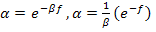 | (1) |
Looking back at the opt-aiNet theory in[13] and CLON- AlG in[3], both theory seems to have one thing in common which is the α, mutation rate. As shown Equation1, the affinity maturation is inversely proportional to the fitness value. This was also stated in[14]. So by increasing the affinity maturation, the cloning rate becomes higher thus rapid mutation rate takes place which is known as hypermutation. Each clones generated have much higher modulation and response compared to their parent cells.This ensures the mutation rate an exceptional selection in one the properties that is chosen for hybrid purpose and also plays an important role for CLONALPropagation. This will be discussed in later chapters. It is important to understand that affinity maturation effects the whole population of clones as one and each clone will have more wider searching capability for local optima. Looking back at[5], this theory can be seen in the selection stage where the candidates are chosen within an allowed boundary. This ensures that value for the chosen candidates maintains its limitation which will then effect the changes in the fitness, f value. A higher value on the clone increases the fitness, f value with respect to the α, maturation rate or affinity maturation value. So by taking this theory into consideration it is also wise to say that the maturation rate equation in Equation 1 would also be able to increase the recognition rate if the value of each clone in the ANN back propagation network is large.
2.2 ANN Back Propagation Modules
ANN strictly functions on both back propagation and feed-forward network. What makes the difference between the two functions is that back propagation focuses on the error signal produced from the difference of actual and desired response[15] while feed-forward network feeds the actual response that propagates throughout the layers of networks[15]. For better understanding, each process of propagation is divided into two sections to perform task given. It involves two important processes, back propagation and feed- forward network as discussed earlier.From there the flow goes in to the next level which per- forms the updates on the system known as the weight updating stage. Each output and input is multiplied to capture the weights maximum direction field for each weight- synapse in this second phase. Along the way, the weights for the opposite direction are deducted from the previous weights captured before. This deduction is also known as the ratio for both opposite and maximum direction which in turn changes the learning rate. Each time a huge difference is detected in the flow, the error increases on that spot and will be amended on the opposite direction. This cycle will be repeated until the network performance is satisfied.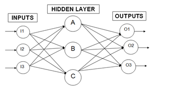 | Figure 1. Back Propagation technique with multiple networks |
Figure 1 shows how a back propagation technique functions does. There are 3 parts to go by starting from the input to the hidden layer and ending with the output layer. Each of these networks is connected through neurons that hold the inputs and outputs respectively. Taking the pattern recognition for example, the process usually kicks off at the input layer. For example, a trained output is predefined as 0 1 0 which acts as the target output. Based on Figure 1, there are three inputs and outputs each represented as I1, I2, I3, O1, O2 and O3. So the target output O1, O2 and O3 should contain all those predefined values in the end. Back to the input layer, the initialization phase starts by calibrating the weights to small random numbers ranging from -1 to 1. Weights are the lines connected from one neuron to another as shown in Figure 1.The input neurons are pumped in with some trained values at the beginning phase. By evaluating the output, O1, O2 and O3 produces different results compared to the target output and this stage is known as the forward-pass network. Usually this is a known result for any first attempt due to the fact that weights are randomly generated. Thus by evaluating the error will then bring the output results much more closely to the target output. Once the known error is evaluated it will alter the weights values so that in each cycle the error produced will get smaller. By doing so, the target output can be achieved and this process is known as reverse pass. This process continues on until a minimal reading for the error is achieved. The error is evaluated using Equation 2. Based on this equation the Output (1-Output) will always refer to the Sigmoid or Transfer Function. A further explanation will be explained on the Transfer Function in the next chapter. A threshold neuron is represented by the extended (Target - Output) function. Threshold neuron is activated when the number of signals given aggravates the inputs making it larger than the inner inputs of the neuron network. | (2) |
3. CLONALPropagation Customization
Altering the nature of both techniques requires a careful study on where they should merge. Both techniques must fit together not just for the purpose of getting a result but also to achieve a better result. This chapter discusses on how the changes are made on both CLONALNet and ANN back propagation.
3.1 Weights and Transfer Function
Looking back at the foundation of neuron networks, ANN incorporates two of the most important compo- nents in neural network which is synapse and neurones. Neurones represents the input nodes while the synapse acts as the output nodes known as weights. Weights are often multiplied with the inputs and summed up. For example inputs are represented with x1 .....xn while weights w1 .....wn which are summed up to producing output O shown in Equation 3.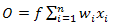 | (3) |
As in Figure 1, the weights are the lines connected to each neurons in the hidden layer consisting of A, B and C. So the weights are represented by WI1B, WI2B and WI3B with respect to neuron B. Then these weights are summed up as shown in Equation 2.The f usually refers to the active function or known as transfer function. Most back propagation algorithm prefers the sigmoid function shown in Equation 4. A sigmoid function is used typically to detect any loss or rejects in a system. In this case, the error rate can be determined by using the sigmoid function. It was first used in Neuron Network and then being transferred into a sensitivityanalysis software known as Brain-Cel. From there, many applications started to implement this function such as in[8] where it mentioned the Multi-layer Perceptron or MLP.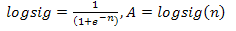 | (4) |
3.2 Algorithm Design
In a process that computes thousands of inputs and outputs it is crucial for an algorithm to deliver an accurate result in short time. To meet that purpose, a combination of both CLONALNet and ANN back propagation is made. Illustrated in Figure 3 is the flowchart of CLONALPropagation starting from the initializing of the training output pattern and ending with displaying all the required parameter outputs. For the first phase, training outputs are defined as shown in Figure 2 where T represents the target output. However they are represented by binary numbers of 1’s for bright spots and 0’s for dark spots.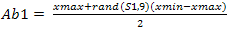 | (5) |
 | (6) |
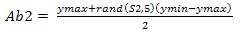
According to[5], the generation of random population as shown in Equation 5 and 6 are initialized at the beginning process. Random population is generated to populate the environment with both strong and weak antibody pools. In this case, values that are generated are within boundary of 1 and -1 with respect to the value given for xmax, ymax, xmin and ymin. Ab1 and Ab2 are the random values taken which will be multi- plied with the weights to form the weights calibration unit as shown in Equation 7.S1 and S2 are two groups of inputs with predefined values of 5 and 3. So by including these values into the equation it will produce matrix groups of (5 x 9) and (3 x 5) which represents Ab1 and Ab2 respectively. The end product matrix will have an output pattern with a (3 x 9) size array because the T, target output size was already set as shown in Figure 3.This ensures that there is variety when the cloning, hypermutation and selection starts. On the back propagation, the random initialization start off with the weights calibration on the input layer as discussed earlier. Thus it is safe to replace the ANN back propagation weight calibration function with CLONALNet’s randomization unit for the second phase. This feature was also explained earlier in the ANN back propagation technique where the weights are calibrated with random numbers ranging from -1 to 1.Following the input initialization phase, the core stage of this algorithm kicks off with the CLONALNet clonal selection process. As stated in[5], the process of cloning, hypermutation and selection starts all in one go. This process is important and complex since only the fittest or the highest values will be selected for the next round. | Figure 2. T as target output |
The first phase of clonal selection takes place with the weights calibration as discussed earlier. Here the inputs Ab1 and Ab2 are multiplied with the weights Ab and A1 as shown in Equation 7.As stated in[5], the process of cloning, hypermutation and selection starts all in one go. This process is important and complex since only the fittest or the highest values will be selected for the next round. Ab is already defined as the pattern size which in this case is a (9 x 9) matrix while A1 is evaluated by performing the logsig function for n1 resulting a (5 x 9) matrix. A1 is then multiplied with Ab2 to produce n2 as shown in Equation 7 and in the end this produces a matrix size of (3 x 9) which matches the T, target output’s size. To achieve the cloning and hypermutation stage, the n2 is then multiplied back with Ab which is the reference value for the input values. From here the value for the clones is achieved and can be used as the parameter in determining the hyper- mutation rate shown in Equation 1. Once this is done, the selection phase starts.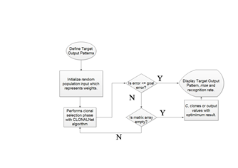 | Figure 3. CLONALPropagation flow chart |
Before that could take place, a preset threshold value is defined which represents the (goal error) shown in Figure 3. Performing this task is important in limiting the clone values from exceeding which in fact gives a better solution since Equation 1 generates outputs based on the value of β. Selection starts by finding the values of nonzero elements inside the pool array. Here each value is compared with the predefined boundary values shown in Equation 5 and 6 consisting of xmax, xmin, ymax and ymin. Each of these values are compared and selected with respect to the conditions whether they are larger than or less than the predefined boundaries. Only those values which meet the condition will be selected and placed in an array represented by outputs Ixmax, Ixmin, Iymax and ymin. From here the real selection starts. These values are normally represented in the form of vectors and vectors have length. For the first step, these pools of arrays are tested to investigate whether they are empty or contain the clones needed.Then the clone vectors are chosen by their maximum lengths. This process will continue on until all the values are collected and matched the (3 x 9) size array of the target output, T. So these values are the pure clones represented by C as shown in Figure 3. | (7) |
The second phase is to evaluate the mse which is the mean squared error. In theory mse or mean squared measures the average squares of errors. It can also be defined as the estimation of error by comparing the real value to the estimated output value. Estimated value is the variance squared divided by the number of generations shown in equation 8.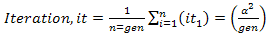 | (8) |
And here the estimated error value is the difference between T and C which results the error rate e. T is the estimated value since it is predefined at earlier stage while C is the real evaluated value from the clonal selection stage. The result from the deduction which is e is then evaluated further more by finding its mean or average. The final value is known as the pure mse rate. These will continue on until the lowest error rate is determined or the number of iteration is met. Either way the result will have a lower mse reading.The third and final phase of the clonal selection is to evaluate the recognition rate. It is important to recognize how accurate is pattern matching as this stage performs that function. As test output values are determined in the end, the wrong rate is evaluated by finding the size of difference between the Target Output, T and test output, TstOutput as shown in Equation 9. TstOutput on the other hand is the real value of C being compared with a predefined threshold value and must always be larger than this threshold value. So a predefined value of 0.5 is given because this value is in the middle of the binary values represented by T, target output. By doing so, each time the evaluation kicks off, values of C which are less than 0.5 will be considered zero while values which are larger than 0.5 will return 1. | (9) |
Finding the recognition rate on the other hand requires the testing images, B which has the same pattern size as Ab which is a (9 x 9) array. The B is also predefined at the beginning of the stage just like Ab but is used as testing parameters while Ab is used during the clonal selection implementation and can said as the training phase. To achieve the recognition rate, size of B to be determined first to ensure that it can deducted with wrong rate shown in Equation 10. Then this result will be multiplied with one hundred because the rate should be in percentage.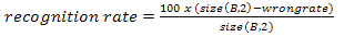 | (10) |
At last all of the output images, mse and recognition rate will be displayed at the output console according to the flowchart sequence in Figure 3.
3.3. Elimination of CLONALNet Steps
At last all of the output images, mse and recognition rate will be displayed at the output console according to the flowchart sequence in Figure 3. As stated in[5], CLONALNet functions as an analyzer rather than dwelling to applications. CLONALNet has the abilities to optimize similar to CLONALPropagation but lacks the capability to be applied in real time scenarios. Furthermore CLONALNet finds the best solution based only on pure clonal selection theory but CLONALPropagation acquires the solutions by both clonal selection back propagation in matching patterns. Looking back at the CLONALNet algorithm shown in[5], the second step which is sorting of the fitness values of individual can be eliminated.The reason is simple because pattern matching do not need the sorting process since the sorting done in CLONALNet requires the Nc or number of clones to be predefined at the beginning stage which acts as a limitation operator. In CLONALNet’s case the sorting is done for the purpose of arranging those clones with higher fitness values from top to bottom. CLONALPropagation however doesn’t initiate the sorting function at the beginning phase since it is taken care of during the weight-updating phase shown in Equation 7. Here each time the n2 is evaluated, A1 will also be evaluated by utilizing in the logsig function. As mentioned earlier the sigmoid function detects loss or errors during the weights calibration. By nature, when this is performed it is already sorting out the best values accordingly following the back propagation rule. Another step which is discarded is the network interaction phase. This step is not required since the interactions between cells are actually the interactions between neurons itself as discussed earlier. It seems in CLONALPropagation each evaluation from the first phase of the algorithm to the end phase requires the interaction of neurons especially during the weights calibration stage.Finally the last step to be eliminated is the insertion of randomly generated clones. Actually this part operates just the same as the second phase of the CLONALPropagation where the C values are rounded up. The only difference here is CLONALNet tends to round it up and insert it one by one. CLONALPropagation on the other hand uses this theory to find the mse and not for insertion purpose. The clones of these neurons are already injected during the selection phase itself.
4. Results and Discussion
The entire outcome of this research is determined in this final part of the work which is the results. In this chapter, results are divided into two sections. First section is represented in the form of graphs. Here both CLONALPropagation and ANN back propagation mse reading and pattern matching is compared. Each comparison is done periodically by increasing the number of generations. For the second section, results are shown in the form of tables where the value of β is utilized only for CLONALPropagation and not in the ANN back propagation technique.
4.1. ANN Output Results
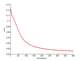
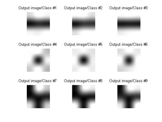
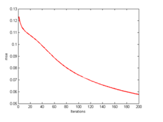
The results from the simulation are divided into four parts of generations for ANN back propagation technique and three parts for CLONALPropagation. Each generation consists of nine output images trained from the algorithm by referring to the T target output. Here the number of generations included for the simulation test is 200, 300, 400 and 500. The purpose is to evaluate pattern recognition rate for each iteration. Included are also the mse reading for each generations for both CLONALNet and CLONALPropagation.The experiment starts off with the 200th generations where the result is shown as in Figure 4. According to the figure shown, the output images from number 1 to 3 seems to have darker spots in the middle and brighter spots above and below. It shows that all the 1’s seems to be concentrating in the middle and the 0’s on above by referring to the T, target output values. This happens because ANN requires additional time to capture the ratio of weights direction field. Here the ratio determines the learning rate performance. Output images from number 4 to 6 does have a significance resemblance to T but still fails to deliver the result. This also goes for the rest of the output images. Base on the mse result shown in Figure 5, the error rate seems to stopped at (0.048). As mentioned earlier due to the lack of additional time, the values of the C are affected as well resulting a poor reading. | Figure 4. ANN at 200th generation |
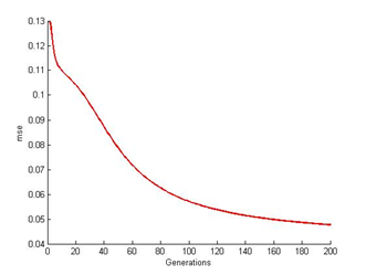 | Figure 5. ANN mse readings at 200th generation |
The optimal result should be a zero error rate. The resemblance seems to occur in the other results as well. Looking at Figure 6, 8 and 10, not only the lack of processing time contributes to the poor result but also the design of the algorithm itself. As mentioned earlier, the algorithm repeats the cycle until its network performance is satisfied. Note that the performance will only reach its peak once the result reaches zero. Its significant enough that this is one of the purpose ANN lacks in system performance.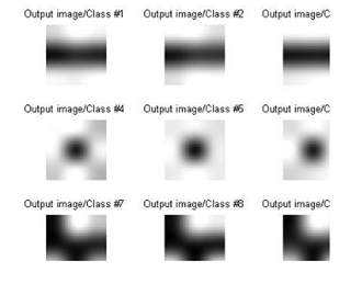 | Figure 6. ANN at 300th generation |
 | Figure 7. ANN mse readings at 300th generation |
 | Figure 8. ANN at 400th generation |
 | Figure 9. ANN mse readings at 400th generation |
 | Figure 10. ANN at 500th generation |
 | Figure 11. ANN mse readings at 500th generation |
4.2. CLONALPropagation Output Results
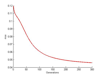
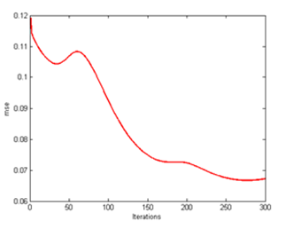
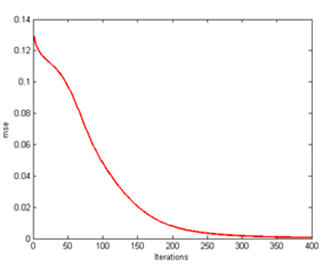
By merging the ANN back propagation technique with CLONALNet clonal selection algorithm, pattern matched according to T data sets have much more accuracy and resemblance. As shown in Figure 12, all the images are assembled accordingly. There are two factors contributing to the accuracy which is the value of the β from the mutation rate equation in Equation 1 and the selection phase itself found in the CLONALPropagation itself.As discussed previously in Equation 1, maturation is inversely proportional to the fitness value stated in[14]. Here the fitness value is actually the C, clones values once it goes into the hypermutation phase. To increase the rate, the value of β must be large which should be defined in the earlier stage itself. The selection phase on the other hand refers to the clonal selection phase of CLONALPropagation whereas mentioned earlier is the task of validating the nonzero elements in pool of arrays. Each time the loop goes by, all the clones which have the maximum length are chosen and each time they have passed this test the algorithm converts it to the real value to meet the target output T. Not only that each time they are converted, they are placed in the order of T where else ANN back propagation doesn’t seem to have.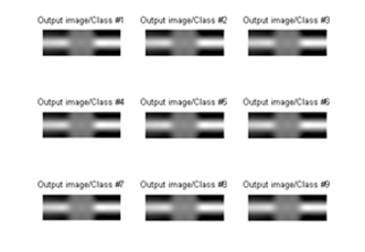 | Figure 12. CLONALPropagation at 200th generation |
 | Figure 13. CLONALPropagation at mse 200th generation |
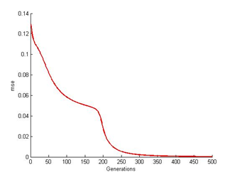
From here, all of these clones are placed in the form of array pool and only those pools which have the exact arrangement will be chosen for the next process. So by performing this function, resources such as processing time and steps are not wasted. Finally a solid image as illustrated in Figure 16 is achieved which resembles the target output T in Figure 2.The mse too improves drastically from one generation to another as shown in Figure 13, 15 and 17. As C values are determined and matched accordingly, the mse improves due to the lower readings of e. The main factor is the increase the C values which affects the e error rate reading after being deducted with T. Following that occurrence, the mse too gets affected as well producing lower mean rate.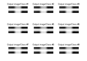 | Figure 14. CLONALPropagation at 300th generation |
 | Figure 15. CLONALPropagation at mse 300th generation |
Finally all that matters is the recognition rate which determines the pattern matching accuracy. Table 1 and 2 shows the after effects with and without the coefficient factor β which explains why the β value is important. Referring to Table 1 of the ANN back propagation technique, the recognition rate seems to be fluctuating. This proves that without the mutation rate from Equation 1 which includes the β parameter must coexist since it controls the number of generations and the maturation rate. 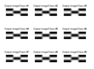 | Figure 16. CLONALPropagation at 400th generation |
 | Figure 17. CLONALPropagation at mse 400th generation |
As for mse evaluation, the same values will be distributed inside the loop for mse rate evaluation. So both evaluations are done simultaneously without interfering the process flow and its performance. Notice that there are no fluctuations in the mse reading in Table 2 and it manages to reach a zero percentage recognition rate.| Table 1. ANN back propagation results without coefficient factor β |
| | No of generation (gen) | mse (mean squared error) | Recognition rate (%) | | 150 | 0.006154 | 22.22 | | 200 | 0.003104 | 33.333 | | 250 | 0.002433 | 44.44 | | 300 | 0.002163 | 66.67 | | 350 | 0.044855 | 33.33 | | 400 | 0.002372 | 77.79 | | 450 | 0.001423 | 100 | | 500 | 0.000886 | 100 | | 550 | 0.000661 | 100 | | 600 | 0.000567 | 100 |
|
|
| Table 2. CLONALPropagation results with coefficient factor β |
| | No of generation (gen) | mse (mean squared error) | Recognition rate (%) | β | | 150 | 0.004964 | 100 | 1 | | 200 | 0.003639 | 100 | 2 | | 250 | 0.001468 | 100 | 3 | | 300 | 0.000447 | 100 | 4 | | 350 | 0.000181 | 100 | 5 | | 400 | 0.000124 | 100 | 6 | | 450 | 0.000115 | 100 | 7 | | 500 | 0.000126 | 100 | 8 | | 550 | 0.0000 | 100 | 9 | | 600 | 0.0000 | 100 | 10 |
|
|
5. Conclusions
Overall CLONALPropagation is an algorithm that doesn’t just operate as an optimizer but also functions in arranging patterns following a predefined set of data. Furthermore CLONALPropagation has the capability to inspect the network performances by utilizing the mse function. Adding to that attribute is the ability to estimate the recognition rate value which is vital in deter- mining the strength of the algorithm. Although CLONALPropagation has all this capabilities, there are still rooms for improvement in certain areas.Further works will be included especially in the development of a frame buffer which acts as an information storage for the data sets. A frame buffer is also a technology used in displaying output from video devices by harnessing information gathered in another buffer known as the memory buffer. This ensure that the stored data sets can be called anywhere throughout the function multiple times without any loss.
ACKNOWLEDGEMENTS
This work is fully funded by the Ministry of Higher Education Malaysia (MOHE) with project code 01101036 FRGS.
References
| [1] | De Castro L.N and Von Zuben F.J, “Learning and Optimization using the Clonal Selection /Principle” IEEE Trans. On Evolutionary Computation, vol.6, pp.239-251, 2002. |
| [2] | Khaled A.Al-Shestawi, H.M. Abdul-Kader and Nabil A. Is- mail, “Artificial Immune Clonal Selection Classification Al- gorithms for Classifying Malware and Benign Process Using API Call Sequences", vol.10, no.1, pp.24-25, 2010. |
| [3] | De Castro, L.N and Timmis .J, " Artificial Immune Systems: A Novel Paradigm to Pattern Recognition ", pp. 3-4, 2002. |
| [4] | Nossal, G. J. V., “The Molecular and Cellular Basis of Affinity Maturation in the Antibody Response, Walter and Eliza Hall Institute of Medical Research”, pp.1-2, 1992. |
| [5] | Jeremiah A.S, Prajndra S.K and Tiong S.K, "Solving Computational Algorithm using CLONALNet Based on Artificial Clonal Selection", in Proceedings of 2011 IEEE Conference on Open System, pp.1-5, 2011. |
| [6] | Jerome H. Carter, “The Immune System as a Model for Pat- tern Recognition and Classification", Journal of the Ameri- cans Medical Informatics Association. vol.7, pp.4-5, 2000. |
| [7] | Liu Ji-zhong and Wang Bo, “AIS Hypermutation Algorithm Based Pattern Recognition and Its Application in Ultra- sonic Defects Detection", in Proceedings of 2005 ICCA International Conference on Control and Automation, pp.1269-1270, 2005. |
| [8] | Jose’ Lima Alexandrino and Edson Costa de Barros Carvalho Filho, “Investigation of a New Artificial Immmune System Model Applied to Pattern Recognition", in Proceedings of 2006 International Conference on Hybrid Intelligent Sys- tems, pp.3-4, 2006. |
| [9] | Jose’ Lima Alexandrino, Edson Costa de Barros Carvalho Filho, “Inverstigation of a New Artificial Immmune System Model Applied to Pattern Recognition", in Proceedings of 2006 International Conference on Hybrid Intelligent Sys- tems, pp.3-4, 2006. |
| [10] | A.Lanaridis, V.Karakasis and A. Stafylopatis, “Clonal Selection-based Neural Classifier ", in Proceedings of 2008 International Conference on Hybrid Intelligent Systems, pp.1-6, 2008. |
| [11] | Bishop, C.M, “Neural Networks for Pattern Recognition Springer, pp.1-477, 2006. |
| [12] | Chaudhari, J.C., “Design of Artificial Back Propagation Neural Network for Drug Pattern Recognition ", International Journal on Computer Science and Engineering (IJCSE), pp.1-6, 2010. |
| [13] | De Castro, L.N and Timmis, J., “An Artificial Immune Network for Multimodal Function Optimization", in Proceedings of 2002 IEEE Congress on Evolutionary Computation (CEC’02), pp.699-674, 2002. |
| [14] | Khaled A.Al-Shestawi, H.M. Abdul-Kader and Nabil A. Is- mail, “Artificial Immune Clonal Selection Algorithms: A Comparative Study of CLONALG, opt-IA, and BCA with Numerical Optimization Problems", IJCSNS International Journal of Computer Science and Network Security, vol.10, no.4, pp.24-29, 2010. |
| [15] | Durai, S. Anna and Saro E. Anna, “Image Compression with Back-Propagation Neural Network using Cumulative Distribution Function", World Academy of Science, Engineering and Technology, vol.17, pp.60-64, 2006. |
 Abstract
 Reference
 Full-Text PDF
 Full-Text HTML