Faruk Alpaslan 1, Erol Eğrioğlu 1, Çağdaş Hakan Aladağ 2, Ebrucan Tiring 1
1Department of Statistics, Ondokuz Mayıs University, Samsun, 55139, Turkey
2Department of Statistics, Hacettepe University, Ankara, 06100, Turkey
Correspondence to: Erol Eğrioğlu , Department of Statistics, Ondokuz Mayıs University, Samsun, 55139, Turkey.
| Email: |  |
Copyright © 2012 Scientific & Academic Publishing. All Rights Reserved.
Abstract
In recent years, artificial neural networks have being successfully used in time series analysis. Using linear methods such as ARIMA and exponential smoothing for non linear time series cannot produce satisfactory results. Although there are various non linear methods, these methods have an important drawback that all of them require a specific model assumption. On the other hand, artificial neural networks have no restrictions such as linearity or model assumptions. In many applications within the time series analysis, it has been seen that artificial neural networks produce more accurate results than those obtained from traditional methods. In spite of the fact that artificial neural networks provide some advantages, researchers keep working on the component selection problem of the method. The answer of the question that which components of the method should be used is a vital issue in terms of forecasting performance. In this study, the effects of number of hidden layer and length of test set on forecasting performance of artificial neural networks are examined. Eight real time series are used in the implementation. The obtained results are analyzed by using statistical analysis and are interpreted.
Keywords:
Artificial Neural Networks, Forecasting, Feed Forward, Length of Test Data
1. Introduction
Artificial neural networks have been preferred in various time series forecasting implementations since its advantages. The most important problem is to determine the right components when artificial neural networks are used for forecasting[1]. When feed forward neural networks are employed, the components of the method such as the number of hidden layer, the number of neurons in the layers, which are input, hidden and in the output layers, the activation functions in the hidden and the output layers and the length of the test set are tried to be determined in order to reach high performance accuracy. To pick right components, different approaches have been used in the literature. The studies until 1998 can be found in[12]. [6,8] examined the number of hidden layer and they claimed that using one hidden layer will be sufficient. Later, [4,13] suggested that two hidden layers should be used to reach more accurate results. According to[5,11], using more than two hidden layers will be useless. In many studies available in the literature, %10, %15, %20 or %30 of time series have been generally used for test set. There is no a general rule to determine the length of the test set. Besides these studies, there have been some studies in which systematical approaches for architecture selection in feed forward artificial neural networks are proposed. [2,3,7] proposed architecture selection methods based on forecasting performance measures. And, [1] proposed an architecture selection approach based on tabu search algorithm.In this study, the answer of the question that “what should be the number of hidden layers and the length of test set to get accurate forecasts?” is searched. To do this, eight real time series which are Ankara air pollution (AAP), Samsun air pollution (SAP), beer consumption in Austria (BCA), airline data series G (ADS), the number of foreign tourists visiting Turkey (FTT), IMKB index (II), exchange rates Turkish Liras/EURO (TLE) and Turkish Liras/DOLAR (TLD) are analyzed and obtained results are examined by using statistical hypothesis. In the next section, brief information about the feed forward neural networks in time series analysis is given. By utilizing tables, Section 3 presents the results obtained from the implementation in which eight real time series are analyzed. In the last section, the obtained results are summarized, interpreted and discussed.
2. Feed Forward Neural Networks
Artificial neural networks approach is a data processing system which mimics biological neural networks. Artificial neural networks can learn from samples included by data. Although the structure of artificial neural networks is simpler than the structure of human neural system, they can produce successful results in various real life problems such as forecasting, classification and image processing.Although different types of neural networks exist in the literature, feed forward neural networks are generally used for forecasting in the applications. Feed forward neural networks consist of layers that are input, hidden and output layers. A broad neural network architecture is presented in Fig. (1). Each layer composes of neurons and neurons are connected with each other with weights. There is no connection between neurons which are in the same layer. In most of studies available in the literature, one neuron is generally employed for output layer. For neurons in hidden and output layers, activation functions are used. The inputs for neurons in hidden and output layers are calculated by summing the values that is obtained by multiplying output values from other neurons by corresponding weights. This summation can be called activation value. Then, the output value of the neuron is obtained by using activation function for a given activation value. Activation function is the non linear part of neural networks and provides non linear mapping. Hence, activation functions which are non linear are preferred for neurons in the hidden layer. For output neuron, both linear and non linear activation functions can be employed.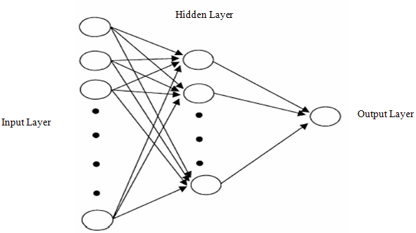 | Figure 1. Multilayer feed forward artificial neural network with one output neuron |
Training process in artificial neural networks can be considered as determining the best weight values that produce results which are most close to target values. Training is performed by optimizing error value according to the weights. In the literature, there are various training algorithms used for training process. One of these algorithms is Levenberg- Marquardt algorithm that has been generally preferred in recent studies. In the implementation, we also use this algorithm for training.In recent years, artificial neural networks have been used in most of the time series applications. The advantages that artificial neural networks have can be given as follows:● Time series can be analyzed without making any test for linearity.● The forecasts which are more accurate than those obtained from traditional methods can be obtained.● Conventional non linear time series methods are not flexible since they were improved for only special non linear structures. On the other hand, artificial neural networks can be used for any non linear time series.● The theory of artificial neural networks is simpler then the theory of conventional approaches so it is simple to utilize artificial neural networks in applications.For both feed forward and feed backward neural networks, it is possible to give forecasting process in seven steps[8].Step 1. Choosing activation function and preprocessing of data.First of all, activation functions that will be used for neurons in hidden and output layers are determined. In our study, logistic activation function given in equation (1) is used in all of the neurons.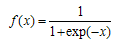 | (1) |
Secondly, observations are mapped into a proper interval in terms of determined type of activation function. If logistic activation function is used, observation values will be mapped into interval[0 1] by using the formula given below.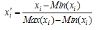 | (2) |
where xi, Max(xi) and Min(xi) represents observation values, minimum and maximum values of observations, respectively.Step 2. Determining the lengths of test and training sets.It is determined that how many percentage of data will be used for testing and training.Step 3. Modeling.The neural network model is determined by selecting the number of hidden layer, the number of neurons in all of the layers, training algorithm (and parameters of that algorithm) and performance measure. Step 4. Generating input values of the neural network.The input values of the neural network are lagged time series. When the input values for time series Xt are generated, m lagged time series Xt-1, Xt-2, . . . , Xt-m are used if m neurons are employed in the input layer.Step 5. Calculating the best weight values.The best weight values are found by using a training algorithm over the test set. Then, the output value of the neural network model is calculated by using the best values of the weights.Step 6. Calculating the performance measure.Predictions for test set are calculated. Then, a transformation which is the reverse of the transformation given in (2) is applied to both the output values obtained in Step 5 and predictions obtained in this step. As a result of this transformation, the calculated values are predictions for training (in sample) and test (out sample) sets, respectively. After this transformation, a performance measure is calculated based on the difference between predictions and real values for test set. In the literature, there are various performance measures that are used to see how good the neural network model could learn the relationships between observations[2]. The most preferred criterion in the applications is root of mean square error (RMSE) and it can be calculated by using the formula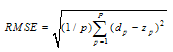 | (3) |
where p, zp and dp represent length of the test set, the output and the target values of the neural network, respectively.Step 7. ForecastingFinally, forecasts for beyond the test set are calculated by using the best weight values obtained in Step 5.
3. Forecasting Results of Feed Forward Neural Networks for Real Data
In order to determine the number of hidden layer and the lengths of training and test sets, time series which are air pollution data for cities Ankara and Samsun (APA and APS), beer consumption in Australia (BCA), Airline Data Seri G (ADS), the international tourism demand of Turkey (TDT), Index 100 in stocks and bonds exchange market of İstanbul (IMKB), exchange rates of Turkish Liras/US dollar (ETU) and Turkish Lira/Euro (ETE) are analyzed by using feed forward neural networks and obtained results are discussed. In the application, two feed forward neural network models given below are used.Model 1: Logistic and linear activation functions are employed for neurons in hidden layer and output layer, respectively.Model 2: Logistic activation function is employed for neurons in both hidden and output layers.1 and 2 hidden layers are employed for each model so four different architectures totally used in the implementation. 10%, 15%, 20% and 30% of time series are taken as length of test set. Thus, each time series is separately analyzed for four different length of test set. When one hidden layer is used, both the numbers of neurons in hidden and input layers are changed between 1 and 12 so 144 architectures are totally examined. When two hidden layers are tried, the number of neurons in input layer is varied from 1 through 12. And, the numbers of both first and second hidden layers are changed between 1 and 3 so 108 architectures are totally examined.In tables in which the results obtained from each time series are summarized, the best architectures that give the best forecasts for test sets and corresponding RMSE values are presented. Architectures with one hidden layer are represented by[n-m-1].[n-m-1] represents an architecture including n and m neurons in input and hidden layers, respectively. For architectures with two hidden layers, the representation[n-m1-m2-1] is employed. In a similar way,[n-m1-m2-1] represents an architecture including n, m1 and m2 neurons in input, first hidden and second hidden layers, respectively. In the implementation, only one neuron is used in output layer for all architectures like done in most of the studies in the literature.In Table 1, the obtained results for APA time series are shown. For first cell of the table ‘8.58[2-7-1]’, when length of test set is 10%, one hidden layer and Model 1 are used, the best architecture is found as[2-7-1] that includes 2 and 7 neurons in input and hidden layers and corresponding RMSE value calculated from this architecture is 8.58.| Table 1. The obtained results for APA time series |
| | | | Percentage of Test Data | | Hidden Layers Number | Models | 10% | 15% | | 1 | Model 1 | 8.58[2-7-1] | 15.35[2-10-1] | | Model 2 | 8.21[12-9-1] | 16.24[1-5-1] | | 2 | Model 1 | 8.56[11-2-1-1] | 11.74[10-2-2-1] | | Model 2 | 7.73[2-3-2-1] | 15.86[2-3-2-1] | | | Percentage of Test Data | | Hidden Layers Number | Models | 20% | 30% | | 1 | Model 1 | 14.61[2-3-1] | 14.78[6-3-1] | | Model 2 | 11.48[10-11-1] | 15.02[6-1-1] | | 2 | Model 1 | 13.12[5-3-1-1] | 14.16[12-2-3-1] | | Model 2 | 15.28[5-1-2-1] | 14.08[6-3-2-1] |
|
|
According to Table 1, for test set length 10%, the best results are obtained when Model 2 with two hidden layers is used. For 15%, the best forecasts are reached when Model 1 with two hidden layers. For 20%, Model 2 with one hidden layer gives the best results. Finally, for 30%, the most accurate forecasts are calculated from Model 2 with two hidden layers. When the obtained results for APA time series presented in Table 1 is examined, it is seen that architectures with two hidden layers generally produce more accurate results. In a similar way, the results obtained from rest of the time series used in the implementation are summarized in Table 2 and 8.| Table 2. The obtained results for BCA time series |
| | | | Percentage of Test Data | | Hidden Layers Number | Models | 10% | 15% | | 1 | Model 1 | 18.17[11-1-1] | 19.26[6-5-1] | | Model 2 | 17.94[4-9-1] | 18.80[7-2-1] | | 2 | Model 1 | 17.88[10-2-3-1] | 18.85[8-3-1-1] | | Model 2 | 18.36[11-2-2-1] | 19.00[8-3-3-1] | | | Percentage of Test Data | | Hidden Layers Number | Models | 20% | 30% | | 1 | Model 1 | 16.43[9-3-1] | 29.03[5-3-1] | | Model 2 | 16.75[7-2-1] | 28.11[7-2-1] | | 2 | Model 1 | 17.39[11-2-1-1] | 27.81[7-2-1-1] | | Model 2 | 17.00[9-3-3-1] | 29.33[3-3-3-1] |
|
|
| Table 3. The obtained results for ADS time series |
| | | | Percentage of Test Data | | Hidden Layers Number | Models | 10% | 15% | | 1 | Model 1 | 0.0472[12-1-1] | 0.0467[11-4-1] | | Model 2 | 0.0629[7-4-1] | 0.06690[6-7-1] | | 2 | Model 1 | 0.0442[12-1-3-1] | 0.0513[12-2-3-1] | | Model 2 | 0.0500[12-1-3-1] | 0.0605[12-1-3-1] | | | Percentage of Test Data | | Hidden Layers Number | Models | 20% | 30% | | 1 | Model 1 | 0.0500[12-1-1] | 0.0588[10-2-1] | | Model 2 | 0.06846[12-12-1] | 0.0818[11-4-1] | | 2 | Model 1 | 0.0504[12-1-1-1] | 0.0478[9-3-3-1] | | Model 2 | 0.0522[9-3-3-1] | 0.0749[11-3-2-1] |
|
|
When Table 3 is examined, it is seen that Model 1 generally gives better results for ADS time series.| Table 4. The obtained results for APS time series |
| | | | Percentage of Test Data | | Hidden Layers Number | Models | 10% | 15% | | 1 | Model 1 | 30.2144[8-5-1] | 36.2506[4-5-1] | | Model 2 | 39.6750[2-1-1] | 35.9797[3-4-1] | | 2 | Model 1 | 32.4994[2-3-1-1] | 37.1699[5-1-1-1] | | Model 2 | 35.6096[5-3-2-1] | 50.3244[2-1-1-1] | | | Percentage of Test Data | | Hidden Layers Number | Models | 20% | 30% | | 1 | Model 1 | 70.8758[9-2-1] | 56.264[12-1-1] | | Model 2 | 66.4199[2-3-1] | 56.6611[8-8-1] | | 2 | Model 1 | 71.7236[9-2-1-1] | 49.4839[6-2-3-1] | | Model 2 | 69.1652[7-1-3-1] | 66.9820[5-3-1-1] |
|
|
According to Table 4, architectures include one hidden layer generally produce more accurate forecasts for APS time series.| Table 5. The obtained results for TDT time series |
| | | | Percentage of Test Data | | Hidden Layers Number | Models | 10% | 15% | | 1 | Model 1 | 105613.2[9-5-1] | 105828.1[9-1-1] | | Model 2 | 116630.8[8-4-1] | 92375.1[8-5-1] | | 2 | Model 1 | 98650.9[7-1-3-1] | 82847.6[8-1-3-1] | | Model 2 | 99407.6[7-1-3-1] | 84954.6[7-1-3-1] | | | Percentage of Test Data | | Hidden Layers Number | Models | 20% | 30% | | 1 | Model 1 | 100491.8[5-1-1] | 111452.4[4-1-1] | | Model 2 | 96482.2[9-3-1] | 93702.7[9-3-1] | | 2 | Model 1 | 86682.9[9-1-3-1] | 231651.5[5-2-2-1] | | Model 2 | 82941.6[8-1-2-1] | 223009.3[5-2-2-1] |
|
|
It is seen from Table 5 that the best results are generally obtained from architectures with two hidden layers for TDT time series.| Table 6. The obtained results for IMKB time series |
| | | | Percentage of Test Data | | Hidden Layers Number | Models | 10% | 15% | | 1 | Model 1 | 1188.5[2-6-1] | 1250.5[1-2-1] | | Model 2 | 1226.2[6-1-1] | 1300.4[1-4-1] | | 2 | Model 1 | 1182.2[11-3-2-1] | 1268.0[5-2-2-1] | | Model 2 | 1091.6[4-2-2-1] | 1309.8[3-1-3-1] | | | Percentage of Test Data | | Hidden Layers Number | Models | 20% | 30% | | 1 | Model 1 | 1018.3[4-2-1] | 973.816[4-2-1] | | Model 2 | 1164.9[1-6-1] | 1002.22[1-10-1] | | 2 | Model 1 | 1184.5[2-1-2-1] | 1035.952[1-3-1-1] | | Model 2 | 1175.6[12-2-2-1] | 1036.385[2-3-2-1] |
|
|
According to Table 6, it can be said that architectures include one hidden layer generally give more accurate results for IMKB time series.| Table 7. The obtained results for ETE time series |
| | | | Percentage of Test Data | | Hidden Layers Number | Models | 10% | 15% | | 1 | Model 1 | 0.0266[1-8-1] | 0.0233[1-5-1] | | Model 2 | 0.0279[1-7-1] | 0.0236[1-5-1] | | 2 | Model 1 | 0.0298[1-3-3-1] | 0.0238[1-3-3-1] | | Model 2 | 0.0284[1-3-2-1] | 0.0240[1-3-2-1] | | | Percentage of Test Data | | Hidden Layers Number | Models | 20% | 30% | | 1 | Model 1 | 0.0219[2-12-1] | 0.0194[1-4-1] | | Model 2 | 0.0218[1-7-1] | 0.0190[1-7-1] | | 2 | Model 1 | 0. 0.02350[1-2-3-1] | 0.01917[1-2-3-1] | | Model 2 | 0.0221[1-3-2-1] | 0.0192[1-3-2-1] |
|
|
When Table 7 is examined, is clearly seen that the best results are obtained from architectures with one hidden layer for ETE time series. In addition, the numbers of neuron in input layers are equal to one for all cases.| Table 8. The obtained results for ETU time series |
| | | | Percentage of Test Data | | Hidden Layers Number | Models | 10% | 15% | | 1 | Model 1 | 0.0109[1-8-1] | 0.0123[1-8-1] | | Model 2 | 0.0096[1-11-1] | 0.0112[1-7-1] | | 2 | Model 1 | 0.0114[8-3-2-1] | 0.0125[1-1-2-1] | | Model 2 | 0.0109[1-3-1-1] | 0.0135[1-3-1-1] | | | Percentage of Test Data | | Hidden Layers Number | Models | 20% | 30% | | 1 | Model 1 | 0.0137[1-8-1] | 0.0116[1-3-1] | | Model 2 | 0.0140[3-1-1] | 0.0109[1-7-1] | | 2 | Model 1 | 0.0135[10-1-3-1] | 0.0111[8-1-3-1] | | Model 2 | 0.0135[1-3-1-1] | 0.0114[1-3-3-1] |
|
|
It can be said from Table 8 that Model 2 generally produces better results than those obtained from Model 1 for ETU time series. Besides this, architectures have one neuron in input layer are generally selected as best architecture.The best architectures that give the best forecasts are presented in Table 1 and 8. When these tables were interpreted, statistical hypotheses were not used. However, Model 1 is compared to Model 2 and architecture with one hidden layer is compared to architecture with two hidden layers in Table 9 by utilizing Mann-Whitney U nonparametric hypothesis test. RMSE values obtained from different architectures for each time series compose the sample for hypothesis test. For instance, APA time series was analyzed with 252 architectures as mentioned before. 252 RMSE values belong to these architectures are compared by using Mann-Whitney U test. The reason of using a nonparametric hypothesis test is that samples do not have Normal Distribution. And, median is preferred as a location parameter.In Table 9, for APA time series, median values are 20.67 and 21.49 for Model 1 and Model 2, respectively. The difference between these models is not significant since corresponding significance probability value obtained from Mann-Whitney U test is 0.101. Therefore, the answer of the question “Is the difference between two models significant?” is ‘No’. In other words, choosing Model 1 or Model 2 will not change the obtained results. In a similar way, the other results given in Table 9 can be examined. For five time series ADS, APS, TDT, IMKB and ETU, the difference between Model 1 and Model 2 is significant. Using Model 1 will give better results for ADS time series while preferring Model 2 will produce better results for APS, TDT, IMKB and ETU time series.According to Table 9, it is obvious that for all time series, the difference between architectures with one hidden layer and two hidden layers is significant since all of the significance probability values are very close to zero. Architectures with two hidden layers produce more accurate forecasts than those obtained from architectures with one hidden layer for all eight time series.| Table 9. Mann-Whitney U test results |
| | Data | Model | Hidden Layer Number | | Model 1 | Model 2 | 1 | 2 | | APA | Medians | 20.67 | 21.49 | 25.63 | 18.32 | | | Decision | No (p=0.101) | Yes (p=0.000) | | BCA | Medians | 27.93 | 28.14 | 35.84 | 24.04 | | | Decision | No (p=0.058) | Yes (p=0.000) | | ADS | Medians | 0.107 | 0.1184 | 0,1143 | 0.1100 | | | Decision | Yes (p=0.000) | Yes (p=0.000) | | APS | Medians | 160.52 | 125.64 | 153.38 | 110.19 | | | Decision | Yes (p=0.000) | Yes (p=0.000) | | TDT | Medians | 207797 | 180771 | 223380 | 158339 | | | Decision | Yes (p=0.000) | Yes (p=0.000) | | IMKB | Medians | 2321.04 | 1915.57 | 3119.72 | 1449.43 | | | Decision | Yes (p=0.000) | Yes (p=0.000) | | ETE | Medians | 0.0454 | 0.049 | 0.0659 | 0.0388 | | | Decision | No (p=0.051) | Yes (p=0.000) | | ETU | Medians | 0.02031 | 0.01938 | 0.0268 | 0.01652 | | | Decision | Yes (p=0.002) | Yes (p=0.000) |
|
|
4. Conclusions and Discussions
Eight real time series are analyzed with feed forward neural networks. Different test set lengths, different types of activation functions and architectures with one and two hidden layers are used in this study. The obtained results are examined by using Mann-Whitney U nonparametric hypothesis test. As a result of the study, it can be said that Model 1 gives better results than those obtained from Model 2 for four data sets. In addition, it is seen that the length of test set has an important effect on forecasting performance. The smaller the test set length is, the more accurate the obtained forecasts are. Another finding is that using architectures with two hidden layers gives more accurate results than those obtained from architectures with one hidden layer for all of the time series used in the implementation.
References
| [1] | Aladag, C.H., "A new architecture selection method based on tabu search for artificial neural networks," Expert Systems with Applications 38( 4) (2011) pp:3287-3293. |
| [2] | Aladag, C.H., Egrioglu, E., Gunay, S., Basaran, M.A., "Improving weighted information criterion by using optimization," Journal of Computational and Applied Mathematics, 233 (2010) pp:2683-2687. |
| [3] | Aladag, C.H., Egrioglu, E., Gunay, S., "A New Architecture Selection Strategy in Solving Seasonal Autoregressive Time Series by Artificial Neural Networks," Hacettepe Journal of Mathematics and Statistics 37(2) (2008) pp: 185-200. |
| [4] | Barron, A.R., "A comment on ‘Neural networks: A review from a statistical perspective," Statistical Science 9 (1) (1994) pp: 33–35. |
| [5] | Cybenko, G. "Continuous Valued Neural Networks with Two Hidden Layers are Sufficient", Technical Report, Tuft University, (1988). |
| [6] | Cybenko, G., "Approximation by superpositions of a sigmoi-dal function," Mathematical Control Signals Systems 2 (1989) pp: 303–314. |
| [7] | Egrioglu, E., Aladag, C.H., Gunay, S., "A New Model Selection Strategy In Artificial Neural Network," Applied Mathematics and Computation 195 (2008) pp:591-597. |
| [8] | Gunay, S., Egrioglu, E., Aladag, C.H., "Introduction to single variable time series analysis," Hacettepe University Press, (2007). |
| [9] | Hornik, K., Stinchcombe, M., White, H., "Multilayer feedforward networks are universal approximators," Neural Networks 2 (1989) pp:359–366. |
| [10] | Lachtermacher, G., Fuller, J., D., "Backpropagation in time series forecasting," Journal of Forecasting 14 (1995) pp:381-393. |
| [11] | Lippmann, R.P., "An introduction to computing with neural nets", IEEE ASSP Magazine April (1987) pp:4–22. |
| [12] | Zhang, G., Patuwo, B.E. and Hu, Y.M., "Forecasting with artificial neural networks: The state of the art," International Journal of Forecasting 14(1998) pp:35-62. |
| [13] | Zhang, X., "Time series analysis and prediction by neural Networks," Optimization Methods and Software 4 (1994) pp:151–170. |
 Abstract
 Reference
 Full-Text PDF
 Full-Text HTML