1. Introduction

One of the most prominent and direct ways that humans have impacted the earth’s surface, across the past 200 years, is through agriculture. Agriculture can be attributed to one of the most important steps and practices in human history, and its role has not diminished in relation to humans as time has gone on (Lev-Yadun et al., 2000). Agriculture has not only played a role in allowing humans to settle in one place and to sustain them, but also plays a large economic role as well. Humans have altered the earth’s landscape for many reasons, but none as much as agriculture. Agriculture represents the largest anthropogenic use of land on earth’s surface (Ramankutty et al., 2008). At the global scale, the production of agriculture has increased faster than population in recent years (Hazell & Wood, 2008).

Considering this level of human and environment interaction and taking into account one of the goals of geography which is to measure such interactions; understanding agriculture through the lens of geography is a critical analysis and of increasing import as conversion continues. Of course, the magnitude of these impacts and roles can be examined and analyzed at different scales; such as global, regional, or local; all with differing results depending on the context of the parameters for analysis. With such a large influence on humans and their environment, not to mention the ample ways to quantify this interaction, it is of paramount importance to accurately measure agriculture.

One of the most important techniques and data sources for quantifying the interaction of humans and their environment is the use of remote sensing. Since remote sensing is used to capture earth’s surface through time, it is one of the most useful tools to determine land cover and land use across the globe. With the recent dramatic increase in the availability of satellite-based products for the large-scale study of various land covers, it is now much easier to monitor agricultural cover at a finer temporal and spatial scale. Climate and soil, land classification and crop inventories, productivity, as well as crop stress and disease are a few areas remote sensing has direct applications to in agriculture (Steven & Clark, 2013).

The use of remote sensing has largely been considered critical for mapping and quantifying change. One of the most applied techniques for land-cover/land-use is the classification of satellite images into land cover maps. There are a plethora of classification techniques used to classify an image. These classification techniques generally fall into either unsupervised classification or supervised classification. Much more recently, machine-learning algorithms have become some of the most prominent methods of classification. One such machine-learning algorithm is Random Forest. A benefit of using Random Forest to classify an image is this technique generally has a higher accuracy than other traditional classification approaches. With this technique, a wide variety of variables are able to be used and Random Forest will ignore insignificant covariates. Random Forest has the great advantage of not overfitting data. This is due to the large number of trees Random Forest “grows” for analysis. This makes Random Forest an ideal classifier for classifying highly complex and heterogeneous landscapes.

It is increasingly important to have accurate and current estimates of crop area and amounts, including crop type, spatial arrangement, and location, for the analysis of food production, biodiversity, agricultural pests and diseases and their related inputs, agricultural policy and land management. Indeed, it is the mission of the National Agricultural Statistics Services (NASS) which is part of the US Department of Agriculture (USDA) to produce such data at an annual timestep for just these reasons (Johnson & Mueller, 2010). NASS produces the Cropland Data Layer (CDL) product which is a raster based, georeferenced, land cover map of crop type. The data is created based on moderate resolution satellite imagery, USDA collected ground control data and the National Land Cover Dataset along with other ancillary products (see Boryan et al. 2011, for detailed description of NASS CRL products). Published analysis of the 2009 products describe accuracies of 85-95% for the major crop categories. Despite these published accuracies, and especially given the importance of the crop type information at the field level, many other researchers have found significant discrepancies between the actual crop covers and the CDL products for their regions of interest, with some areas experiencing over or underestimations of 50% (Larsen et al, 2015). As such, it is deemed essential to review the CDL products for specific regions of interest prior to their use within any research studies.

While these concepts of quantifying human and environment interaction through land-cover/land-use change via remotely sensed image classification can be applied anywhere on earth and at a multiscale level; for example, a global, regional, local, or other scale; this research will focus on a state scale level with an emphasis on the top agricultural crops in Florida. This research looks to improve upon current methods used to identify and estimate areas in different agricultural crops and to better determine changes in agricultural crops over time in the state. The research objective is to develop an integrated high resolution and Landsat based remotely sensed analysis to understand the spatial and temporal pattern of the top five crops in Florida. Specifically, this research aims to: (1) develop a random forest classification which integrates both spatial and temporal data to estimate agricultural crop areas in Florida, (2) to compare these results with the federally published data and field data to determine which method is better, and (3) to map the areas in citrus, cotton, peanut, sugarcane and strawberry and determine area and location of change between 2008 and 2016. The result from this research will hopefully assist agriculture and land managers alike, with consideration to higher accuracy for three key areas: location, quantity, and agriculture type.

2. Materials and Methods

2.1. Study Area

Determining area and extent of crop coverage across the state is of key importance for economic and environmental concerns. The top five crops in Florida are Citrus, Sugarcane, Strawberry, Peanut and Cotton. Florida has a total area of 170,310 km2 and hosts a rich agricultural diversity. According to the USDA and NASS, oranges are so important to the state of Florida that in 2016 they generated $905,138,000 in the value of production. The next most profitable crops are grapefruit ($136,495,000), and hay ($129,600,000) (United States Department of Agriculture, 2016). In 2015, Florida produced 60% and 58% of the total value in the United States for oranges and grapefruit, respectively, according to the Florida Department of Agriculture and Consumer Services (Florida Department of Agriculture and Consumer Services, 2017) and as such, citrus is a key crop across the state (Boriss, 2007). Florida also produces 54% of the US value in sugarcane for sugar and seed production, valuing at $515 million, as well as 13% of strawberries, valuing at $291 million (United States Department of Agriculture, 2016). Other prominent crops in the state are peanuts and cotton. As such, Florida is the top producer nationally of oranges and sugarcane and economically speaking, in 2014, almost 14% of all jobs in the state were linked to agriculture, with $155 billion from direct industry output and $127.3 billion in value-added contributions. In 2017 Florida had 47,000 farm operations covering 9.45 million acres of farmland which was another year of decline, from its peak of 48,000 farms covering 9.55 million acres in 2013 (University of Florida IFAS, 2017). Accuracy in the location, amount and type of crops, as well as changes in production over time, is therefore of key interest to land managers and the state overall.

Various researchers have highlighted limitations of existing agricultural data sources (Lark et al. 2017, Rahman et al. 2019), specifically the use of the USDA/NASS CDL product, which is also widely recognized as the best available national level data. As such, given our interest is in location, extent and change in the top five crops between 2008 to 2016, we created two land cover classifications based on field data, and then compared these results and the CDL product to determine if our product outperforms the existing nationally and most widely used crop product available. Using field sites, visited by our team, we determined the accuracy of both products and determined changes in the top five crops for the state of Florida between the time periods of interest.

2.2. Remote Sensing Data

The remotely sensed imagery used in this study was obtained from the Landsat-ETM+ (Enhanced Thematic Mapper Plus) sensor as well as the Landsat-OLI/TIRS (Operational Land Imager/Thermal Infrared Sensor). These sensors obtain imagery at a 30 m spatial resolution for most bands, save for the thermal band on the ETM+ sensor which has a spatial resolution of 60 m and the thermal infrared bands on the OLI/TIRS sensors that have a spatial resolution of 100 m. Both satellite platforms have a temporal resolution of 16 days.

When creating classifications of agricultural landscapes, it is essential to account for the crop calendar for each crop being grown. Specifically, this helps identify ideal times to be able to extract land cover information in order to differentiate crop types, determine grassland from agricultural fields and highlight citrus versus seasonal crops. The full suite of available imagery was first analyzed, and five dates selected for each crop that most clearly differentiated the different crop types from their surrounding landscapes. Based on differences in crop types and their related growing patterns, the selected dates differed by crop (Fig. 1 and Fig. 2). The resultant crop calendar graphs by spectral signature for the imagery used in this study, highlights times of differentiation and also shows variation in signatures throughout the growing seasons. This information was compiled across all five crop types and the best image dates were selected to differentiate crop landscapes and types. The growing seasons and distinguishable development points for each of the five key crops spanned the entire calendar year. Development points for the crops included stages such as planting, emerging, budding, flowering, fruiting, and harvesting. These stages were not identical between the five crops and so the need for multiple image dates, rather than only one or two, to best represent the range of growing conditions for all crops studied. This resulted in the creation of two composites of the different growing periods, for 2008 and 2016. In these composites, all five different dates throughout the growing season were used to create a single image stack of each year’s composite (Table 1, Fig. 1 and Fig. 2). There was an attempt to keep month and days consistent between the two years, but due to the temporal resolution of the satellite, as well as image quality when considering variables such as cloud coverage and growing days, slight deviations were made when selecting exact dates for each of the year’s composites.

Table 1. Landsat image dates used for the random forest classification of crop type

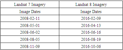
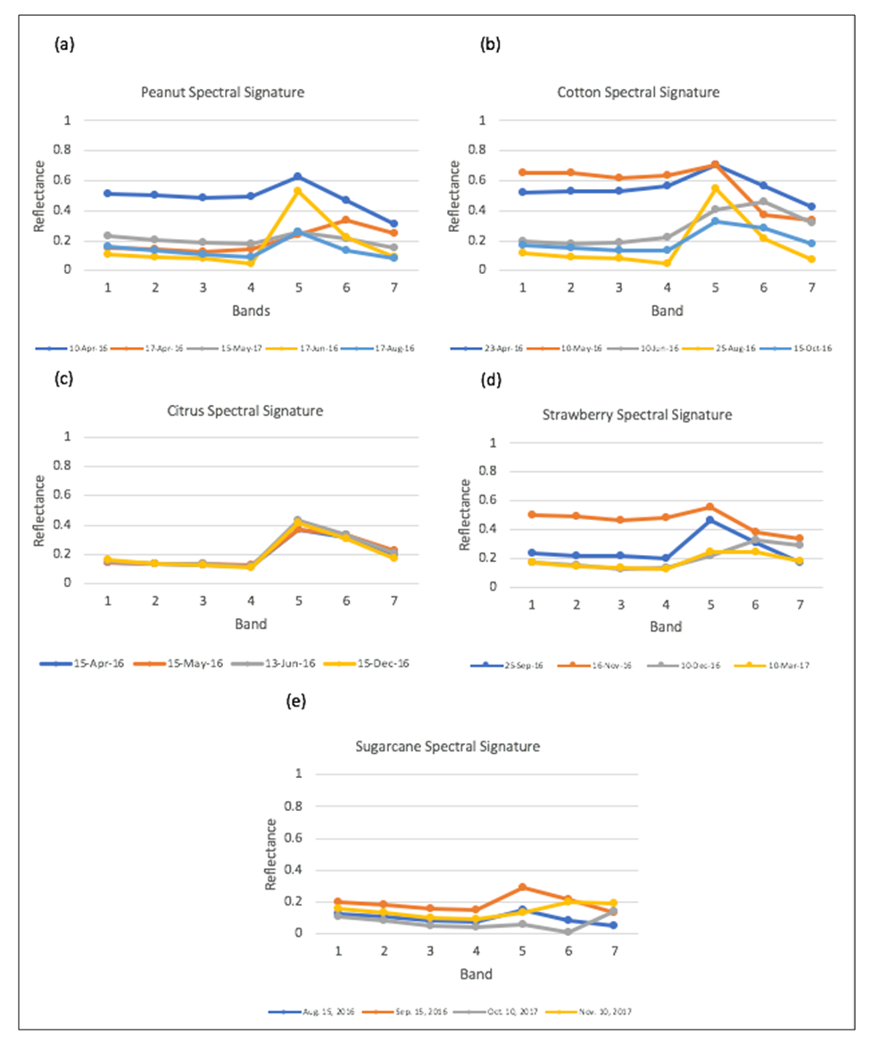Figure 1. Spectral signatures of (a) peanut, (b) cotton, (c) citrus, (d) strawberry, and (e) sugarcane for Landsat at different development points within the growing season

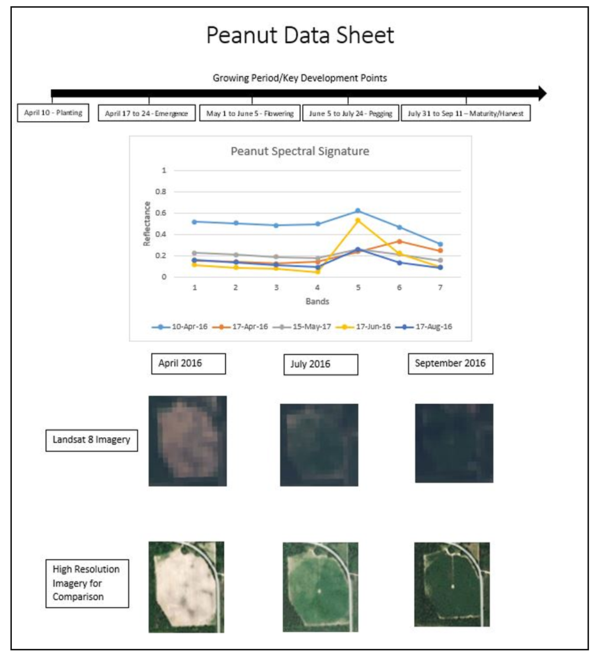Figure 2. Crop calendar information for Peanuts in Florida, with related spectral signature plot for Landsat 8 data, and their high-resolution Google Earth image and Landsat image views over time for an example calibration peanut site location

In addition to the individual Landsat image bands a series of spectral indices were created to highlight differences in vegetated surfaces. These included the Normalized Difference Vegetation Index (NDVI), Normalized Difference Wetness Index (NDWI), and Enhanced Vegetation Index (EVI). NDVI and EVI are commonly used indices to highlight vegetation growth, vigor and health and in association with the NDWI are excellent at highlighting slight changes in vegetation cover, growth and health (Beck et al. 2011). As such, they can separate crop types across the growing season and also to differentiate crops from other natural land cover types within the state. Therefore, the input data for the classifications included the multiple image dates for bands with the created additional indices.

The classification was performed in two stages. In the first stage this study analyzed the full suite of land cover data for the state. This scheme included 12 classes. The classes consisted of the five key crops of cotton, citrus, peanuts, strawberries, and sugarcane and seven additional classes of urban, forest, grassland, woody wetland, herbaceous wetland, shrubland, and fallow. These latter seven classes were selected because they represented at least 1% of Florida’s land cover, according to the CDL. To create the reference data for the classifications, random samples were collected during both years of interest. For 2016, a total of 833 reference data points were generated for the 12 classes. In 2008 a total of 725 reference date points were created. Given most agricultural land in the state has been in its designated cover for some time, most changes were in cropping type or rotation within a given year or abandonment of areas formerly in agriculture. As such, the 12 classes were reduced to only those classes of interest: the class of agricultural land, and specifically to the 5 main crops of interest. This allowed for improved accuracy of classification, and reduced confusion of classes not part of the agricultural landscape. As such, the classification only addressed changes in crop type within known agricultural lands within the state, from 2008 to 2016.

An ensemble learning method was used for the supervised classification. Random Forest (RF) is an advanced machine-learning algorithm that does not require parametric assumptions to be made (Breiman, 2001). This method is widely-used because it tends not to overfit data and has been shown to work at a high degree of accuracy even in complex systems . Generally, RF performs well compared to other supervised classification techniques. The reason random forest and tree voting works is through the use of the Strong Law of Large Numbers so the classifications converge and overfitting is reduced as a problem (Breiman, 2001). This technique uses the variables in many statistical trees in which the variables at different branching nodes randomly mutate and each tree ‘votes’ for the potentially most popular class (Breiman, 2001). 80% of reference points were used for training the RF classifier and the remaining 20% were used for accuracy assessment.

2.3. USDA’s Cropland Data Layer (CDL)

The most readily available crop coverage estimates were the national crop coverage generated by the USDA. The USDA’s CDL contains information on land cover across all states, focusing specifically on the most dominant crop types nationally (United States Department of Agriculture, Cropscape - Cropland Data Layer 2017). The CDL is a raster, geo-referenced, crop-specific land cover data layer created annually for the continental United States using moderate resolution satellite imagery and extensive agricultural ground truth data (United States Department of Agriculture, About CDL 2017). Originally released at a 56 m resolution, the 2008 CDL was reprocessed using Landsat 5 Thematic Mapper data and released at a 30 m resolution. The 2016 CDL utilized imagery from Deimos-1, UK-DMC 2, and Landsat 8 to produce a 30 m resolution product for the continental United States (United States Department of Agriculture, About CDL 2017). The CDL has been used for many real-world applications, ranging from disaster assessments to agricultural policy decisions (Reitsma et al., 2015). As such, the CDL products for 2008 and 2016 were downloaded and mapped to compare our own satellite based classified products too.

In addition, the USDA NASS’s Quick Stats portal also gives crop coverage in acres at multiple geographic scales including national, state-level, and county-level (United States Department of Agriculture, USDA/NASS QuickStats Ad-hoc Query Tool 2017). The Quick Stats coverage data is not geo-referenced data, but rather is a numerical product in which some level of accuracy analysis has been undertaken and corrections attempted to improve the CDL product. As such, many researchers use the NASS estimates as a more realistic validation of the actual acreage in each crop at a state level. Given this, we also extracted the NASS data for each crop for the state of Florida, for comparison, numerically, with our own satellite derived land cover classification product.

3. Results

3.1. Classification of the Top Five Crop Types

To assess the accuracy of the classification, a total of 250 sites, 50 sites for each of the five crops, were randomly selected to be ground-truthed. For 2016, of the 250 ground-truthing sites, a subset of 80 sites was physically visited. The remaining 170 sites were verified using high-resolution satellite imagery. Using approximately 25% validation data, from the created reference data points for each year, accuracy assessments were completed, with confusion matrixes, for both the 2016 and 2008 random forest crop classifications. For both years, the overall accuracy of the random forest classifier was over 85%. In the 2008 classification, the accuracy for the validation data is 89.9%. In the 2016 classification, the validation accuracy is 86.5%. The resultant crop coverage maps for Florida for 2008 and 2016 indicated that crop locations are spatially distinct across the state (Fig. 3) with set zones of different agricultural growth regions, reflecting the climatic and biotic conditions across the state.

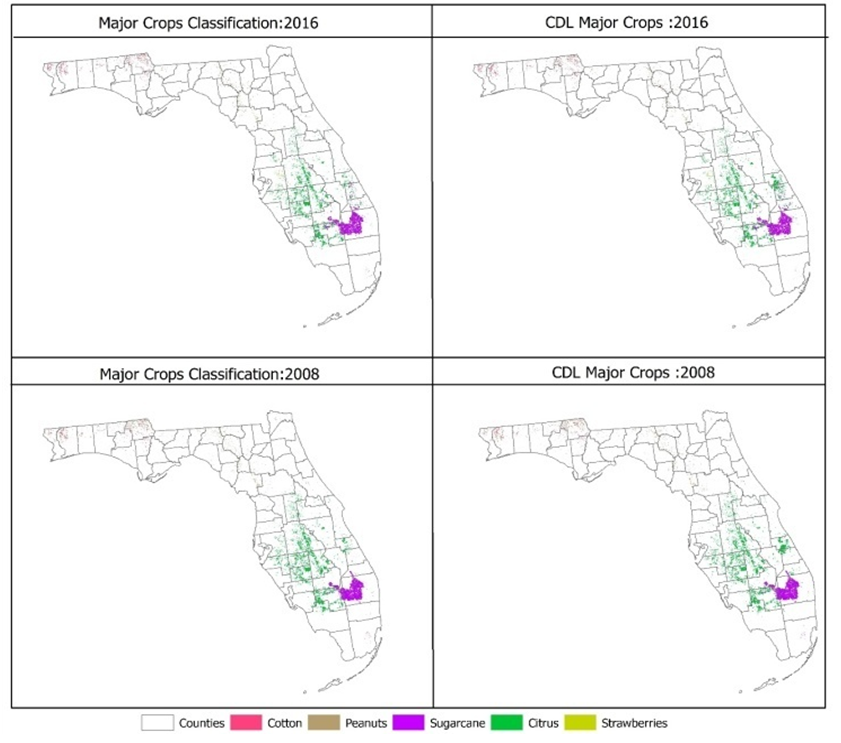Figure 3. Top five crop classification from the random forest on the left and on the right map presents The USDA Cropland Data Layer classification for the five key crops in Florida for 2008 and 2016

When looking at the change in crop area over the two dates of analysis the overall, total acreage for the five crops has been stable, with only a relatively small decrease (4.17%), from 5,571.88 km² to 5,339.71 km², between 2008 and 2016. Citrus, sugarcane, and peanut are the most common crops for both periods, while cotton and strawberry crops accounted for a small portion of the total acreage. The acreage change for cotton, citrus, and strawberry were substantial. Citrus acreage decreased by 12.43% from 3,016.51 km² to 2,641.69 km². Cotton acreage increased by 50.19% from 236.12 km² to 354.63 km². The largest percent of acreage increase was observed for strawberry, from 1.45 km² to 23.72 km². Sugarcane and peanut crops experienced small acreage changes. Sugarcane acreage increased by 2.15%, from 1,615.03 km² to 1,649.79 km², while peanut acreage decreased by 4.68%, from 702.74 km² to 669.87 km².

Table 2. Change in crop area from 2008 to 2016 across Florida in km2

3.2. USDA’s Cropland Data Layer Assessment

To assess the accuracy of the USDA’s Cropland Data layer with our classification, and utilized the same 250 sites, 50 sites for each of the five crops, to test the actual crop type based on the field visits and high-resolution imagery, to the CDL product. From the 250 sites, a total of 87 sites were accurately classified by the USDA CDL for a 34.8% overall accuracy. The same 250 sites were used for 2008 and verified through imagery. The accuracy for 2008 was 32.4%.

3.3. Comparison of RF Classification, CDL and NASS Statistics

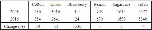
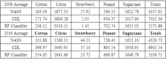
This study compared the two raster based spatial products, along with the USDA NASS data which is the adjusted CDL estimate. There were differences between the CDL and official NASS estimates for acreage statistics because CDL estimates depend upon pixel counting. Pixel counting is usually downward biased when compared to the official estimates. The bias is corrected via regression methods that are applied and generates the official NASS data. As such, in this analysis we are comparing the CDL raw data, the NASS official statistics and the RF classification produced in our research. In this way we hope to account for any possible error in the CDL product by also including the regression corrected NASS data.

Crop acreage coverages from the random forest classifications are compared with both the USDA’s CDL classification, and the NASS’ official acreage counts for the specified crop types in Florida (Table 3). When viewing the data (Table 3), with the exception of strawberries, which are massively underestimated by both CDL and the RF classifiers in 2008, the RF classifier produces values much closer to the official NASS statistics than the CDL. Given the NASS data are reportedly based on some regression adjustment of the CDL data this result seems most interesting. Our classifier significantly outperforms the CDL both in terms of the NASS data and in terms of validation. If we select a couple of crop examples to highlight the differences in performance of the CDL versus the RF classifier (Fig. 4) we can clearly see a higher quality and more spatially refined product from the RF classifier than the CDL product.

Table 3. Acreage counts for official NASS estimates, Cropland Data Layer classification estimates, and random forest classification estimate in km2

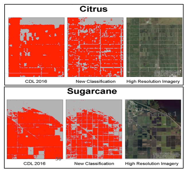Figure 4. Comparison of the CDL and our RF classification products for two known field sites for (a) cotton and (b) sugarcane. The higher resolution imagery is also show to provide a visual comparison of the actual cover to compare both classification products too

3.4. Trajectories of Crop Change from 2008 to 2016 from the RF Classifier

Spatially, there were limited areas of crop changes across the state, totalling less than 4% overall in terms of loss of crop coverages. When we view at a pixel level though we can also identify areas that stayed cropped but had a different crop grown or a rotation in crop type. While there may have been a 5% loss in crop area between 2008 and 2016, there was also a conversion of crop types. For all crops, the majority of area was stable. The largest changes were between peanuts and cotton with 123.3 km² of change and 68.8 km² of change from cotton to peanuts. The next large changes were observed for change from citrus to sugarcane, for 23.9 km², and strawberry, for 6.3 km². The land cover trajectories for the state are given in Table 4, with all areas of conversion, totalling at least 1.0 km² highlighted. Examples highlighting these conversion areas for three sample sites are illustrated visually in Fig. 5.

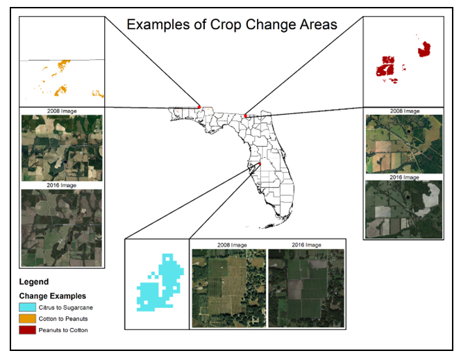Figure 5. Examples of crop change trajectories for three different conversions of citrus in 2008 to strawberries in 2016, cotton in 2008 to peanuts in 2016 and peanuts in 2008 to cotton in 2016. At different locations around the state. High resolution imagery is shown to highlight the on the ground conversion and map inset shows land cover area from the RF classification

4. Discussion

The extent and spatial organization of crops and crop types is of paramount importance in terms of global food production and related areas such as biodiversity, management of pests and diseases within agricultural landscapes and also linked to human health and water quality issues (Larsen et al. 2015).

Geospatial data, especially satellite images, holds the greatest promise for the provision of detailed information on agricultural extent, crop type, and health. Such in-season crop identification is essential for management-based decisions (Rahman et al. 2019). This study found low accuracy of pre-existing national level agricultural data, the USDA CDL product, such as these pixel-level data. The results, when coupled with earlier studies indicate a need for caution given their suite of limitations or possible inaccuracies (Lark et al. 2017).

The random forest classifications yielded 85% overall accuracy for both 2008 and 2016 years, and outperformed the USDA Cropland Data Layer classification with its accuracy of less than 40%. Crop coverage across the state still shows citrus to be the number one crop in terms of area, followed by sugarcane, peanut, cotton and then strawberry. Across the state approximately 4% of the area in agriculture was lost across the study period and the greatest losses in overall crop area were found for citrus (-12%) and peanuts (-5%). Strawberry increased significantly as a percentage, in part due to the, initial, very low area in this crop, and cotton also increased significantly in area. The RF classification was found to be a strong performer in spatial accuracy when compared to actual field visits, and also was closer to the USDA NASS adjusted numbers state-wide, than the CDL product on which the NASS numbers are based. Such low total accuracy for the CDL (30-50%) makes this product unsuitable for use for looking at these crops within our study region, especially in terms of addressing changes in these crop areas over time. The very low levels of accuracy for this product make it unusable in any further studies which need accuracy and spatial location information and make the creation of real crop classification essential for this state. As such, this new RF classification of the top 5 crops for the state of Florida, was found to be a superior product for the study of crop change and also for use in additional studies based on the location and quantity of crops in Florida.

While the CDL holds value when considering agriculture crop coverage at a national scale, especially when considering its high temporal frequency, in that it is completed annually for every state (Han et al., 2014). In this example, it does not hold up at the state scale when considering performance of classifiers and accuracy. The USDA CDL classifications do have a series of known errors but the very low accuracy levels indicated here are well below those reported by other researchers. Reitsma et al (2016) investigated CDL cropland accuracy across South Dakota and found highly variable results over space, with overall accuracy levels between 89.2 and 42.6%. These ranges are variable, but the lower end of accuracy does match our findings within Florida for the five selected crops. Similarly, Larsen et al (2015) found that accuracy was highly variable with over or underestimates of +/- 50% possible. Lark et al (2017) cautioned in their research, the use of CDL data for tracking crop changes over time. Their research found that special considerations were necessary when using the data in this way, specifically they recommended a need to account for crop area underestimation within this dataset. Particularly, the known underestimation of crop area if pixel counts are used from the CDL data directly (Boryan et al., 2011), when compared with data such as the NASS, is such that there is a linear regression model built to correct for this error. While the CDL is clearly a useful and unique dataset, available at an annual timestep, and highly beneficial to many research studies, it can also be problematic and should always be validated with in-situ field data prior to being used for land change studies (Rahman et al. 2019).

Other researchers addressing issues of crop change and comparing to the CDL dataset have also found the random forest classifier to be a superior technique for classification accuracies (Rahman et al. 2019) in comparison to the CDL direct output. In addition to the use of random forest classifiers these researchers also compared the use of single date versus multi-date imagery for crop classification and reported multi-date image incorporation significantly improved the classification accuracy. Incorporating multi-date images across the season within this research, in a single stacked image layer for classification, was clearly superior to a single image date, for agricultural classifications with highly variable coverage within a season.

For land managers and those researchers interested in modelling crop location and area, care must be taken when using national data products such as the CDL. In addition, when interest is focused on only a few crops, it is evident that site specific classifications require extensive field calibration. Use of the CDL products are on the increase (Lark et al. 2017, Han et al. 2012) making research on their accuracy and site-specific applicability also of key importance to researchers. The work discussed here highlights the importance of accurate crop classifications for Florida where declines in the citrus industry and areas under citrus coverage are declining, and different crops, such as cotton, are increasing in area. Such changes, especially when Florida represents the number one producer nationally for Citrus, are of great importance economically to the state and region. The implications of changes in crop distribution and amount, have real impacts on natural resources state-wide, with such agricultural regions and their related management practices which are crop dependent, impacting our water supply, air quality, climate, and wildlife habitats.

5. Conclusions

This research analyzed the changes in agricultural coverage across a set time period within the state of Florida, looking at the top 5 crops in terms of economic importance. This study applied remotely sensed analysis techniques to analyze the crop cover change and compared it to those produced nationally. The results of this research achieved accuracy above 85%, which is a significant improvement compared to the CDL data. A few limitations this study faced were inaccessibility to the CDL methods and training data. With a greater understanding of the exact methods used in the creation of CDL, it would have been easier to improve upon and test this created product. Since the CDL is an annually produced product, the methods are constantly being updated and changed. However, at the time of this research, we were unable to receive the requested information. With more time, a number of improvements could be made to this study. The inclusion of more crop types and land cover types, with more training data could result in even higher accuracy for the random forest classification. Of course, an additional improvement for this study would be to add more training data for the classification. Supplementing the classification with additional training data would likely improve the classification and could improve the results in terms of accuracy. This research highlights the need for field-based geographical research, and the utilization of geospatial analysis tools and advanced remotely sensed methodologies to better understand spatial variation in such important cover types. The tools and approaches geographers can bring to such studies are of paramount importance and such research should be continued and built upon in future work.

ACKNOWLEDGEMENTS

This work is supported by Southeastern and Coastal Center for Agricultural Safety and Health (SECCAgSH)(No. NIOSH/CDC: U54 OH011230).