Haidy Elsayed, Mohamed Zahran, Ayman ElShehaby, Mahmoud Salah
Department of Surveying Engineering, Shoubra Faculty of Engineering, Benha University, 108 Shoubra Street, Cairo, Egypt
Correspondence to: Haidy Elsayed, Department of Surveying Engineering, Shoubra Faculty of Engineering, Benha University, 108 Shoubra Street, Cairo, Egypt.
| Email: |  |
Copyright © 2019 The Author(s). Published by Scientific & Academic Publishing.
This work is licensed under the Creative Commons Attribution International License (CC BY).
http://creativecommons.org/licenses/by/4.0/

Abstract
This research proposed an approach for automatic extraction of buildings from digital aerial imagery and LiDAR data. The building patches are detected from the original image bands, normalized Digital Surface Model (nDSM) and some ancillary data. Support Vector Machines (SVMs) and artificial neural network (ANNs) classifiers have been applied individualey as member classifiers. In order to improve the obtained results, SVMs and ANNs have been combined in serial, parallel and hybrid forms. The results showed that hybrid system has performed the best with an overall accuracy of about 87.211% followed by parallel combination, serial combination, ANNs and SVMs with 84.709, 82.102, 77.605 and 74.288% respectively.
Keywords:
Building extraction, nDSM, Hybrid system, Image classification, SVMs and ANNs
Cite this paper: Haidy Elsayed, Mohamed Zahran, Ayman ElShehaby, Mahmoud Salah, Integrating Modern Classifiers for Improved Building Extraction from Aerial Imagery and LiDAR Data, American Journal of Geographic Information System, Vol. 8 No. 5, 2019, pp. 213-220. doi: 10.5923/j.ajgis.20190805.03.
1. Introduction
Detection and reconstruction of buildings are of high interest in the geospatial community. Traditionally, the building boundaries are delineated through manual digitization from digital images in stereo view using the photogrammetric stereo plotters. However, this process is a tiresome and time-consuming task and requires qualified people and expensive equipment. Thus, building extraction using the automatic techniques has a great potential and importance. Automatic building extraction has become one of the most investigated research topics motivated by the development of high resolution image acquisition and machine learning. While many algorithms have been proposed for building extraction, none of them solve the problem completely. The availability of high resolution aerial imagery and other data sources such as LiDAR data can provide a high quality building extraction. One can make benefits from LiDAR and photogrammetric imagery as each of such data has particular advantages and disadvantages in horizontal and vertical positioning accuracy. Compared with photogrammetric imagery, LiDAR generally provides more accurate height information but less accurate edges. Photogrammetric imagery can provide extensive 2D information such as high-resolution texture and color information as well as 3D information from stereo images. Over the last decade, many researches and development efforts have been put into extracting and reconstructing building from images. Lee et al. [1] proposed a classification-based approach to extract building boundaries from the IKONOS multispectral and panchromatic images. Initially the multispectral image was classified using the ECHO region-based classifier technique. Then, the classified images were vectorized to define the working windows. Finally, the building boundaries were delineated using a building squaring approach, which is based on the Hough transform. Jin and Davis [2] demonstrated an integrated strategy for identifying buildings in 1-meter resolution satellite imagery of urban areas. Buildings are extracted using structural, contextual and spectral information. Three building detectors are applied to a preprocessed PAN image. Two of these detectors are based on a differential morphological profile (DMP) analysis of the preprocessed PAN image. The first detector is mainly based on structural information of the building itself, where buildings hypotheses of relatively large scale are generated from the DMP. Then the hypothesized building components are verified through shape information of the components. The second detector is primarily based on contextual information of the buildings. Shadow hypotheses are generated from narrow dark structures identified in the DMP. Shadow components are verified using spectral characteristics and image collection geometry, and then shadow corners are generated by projection analysis. The third building detector is primarily based on the spectral information of building itself. The objective is to extract bright buildings, especially small ones that are ignored by the other two detectors. ZahraLari and Hamid Ebadi [3] proposed an automated system for extraction of buildings from high-resolution satellite imagery that utilizes structural and spectral information. Using ANNs algorithms, the detection percentage and quality of the building extraction are greatly improved. In the first part, initial image processing and segmentation is done. In the second part, segment’s features are extracted. In the third part, the system decides about possibility of each segment’s being building based on features extracted using ANNs. This system works in two phases: i) learning phase: the neural network presented in third part of system trains using manually saved data to reach desirable accuracy criterion; and ii) application phase: the systems tests on new dataset. Omo-Irabor and O.O [4] studied the changes in the southern part of Nigeria by from 1987 to 2002. They used the ISODATA unsupervised and the supervised Maximum Likelihood classifiers for detecting land use/land cover (LULC) classes. Zhu et al. [5] proposed a classification-based approach for building change detection from digital surface models (DSMs) which are generated from the images acquired by a multi-line digital airborne sensor ADS40. A strategy is proposed that allows efficient integration of a local surface normal angle transform (LSNAT) method and marker-controlled watershed segmentation (MCWS) method for building extraction in urban areas. The LSNAT method uses a hierarchical strategy to extract huge buildings and the MCWS method extract low heights and very small areas. The proposed strategy presents wonderful results for building extraction and acceptable results for change detection compared to some other change detection methods. Woosug Cho et al. [6] proposed a practical method for building detection using airborne laser scanning data. The approach begins with pseudo-grid generation, noise removal, segmentation and grouping for building. Followed by, detection, linearization and simplification of building boundary. At the end, buildings are extracted in 3D vector format. Jiang et al. [7] proposed an object-oriented method to extract building information by DSM and orthoimage. With object-oriented methods, not only the spectral information but also the shape, contextual and semantic information can be used to extract objects. The object-oriented building extraction typically includes several steps: data pre-processing, multi-scale image segmentation, the definition of features used to extract buildings, building extraction, post-processing and accuracy evaluation. Zheng Wang [8] proposed an approach for building extraction and reconstruction from LiDAR data. The approach applied terrain surface data as input data. The process includes edge detection, edge classification, building points extraction, TIN model generation, and building reconstruction. The objective is to extract and reconstruct buildings and building related information. For building detection, it detects edges from the surface data and classifies edges to distinguish building edges from other edges based on their geometry and shapes, including orthogonality, parallelism, circularity and symmetry.Koc San and Turker [9] proposed an approach for the automatic extraction of the rectangular and circular shaped buildings from high resolution satellite imagery using Hough transform. The strategy consists of two main stages: i) building detection and ii) building delineation by Hough transform. The candidate building patches are detected from the imagery using SVMs classification. In addition to original image bands, the Normalized Difference Vegetation Index (NDVI), and nDSM are also used in the classification. After detecting the building patches, their edges are detected by using the Canny edge detector. The edge image is then converted into vector form using the Hough transform. TxominHermosilla et al. [10] presented evaluation and comparison of two main approaches for automatic building detection and localization using high spatial resolution imagery and LiDAR data which are: i) thresholding-based and ii) object-based classification. The thresholding-based approach is founded on the establishment of two threshold values: one refers to the minimum height to be considered as building, defined using the LiDAR data, and the other refers to the presence of vegetation, which is defined according to the spectral response. The other approach follows the standard scheme of object-based image classification: segmentation, feature extraction and selection, and decision trees-based classification. The results obtained show a high efficiency of the proposed methods for building detection, in particular the thresholding-based approach, when the parameters are properly adjusted and adapted to the type of urban landscape considered. Yan Li et al. [11] proposed an integrated method of building extraction using transform from DSM to normal angles and watershed segmentation to the gradient of DSM by using imagery and nDSM with 1m spatial resolution. To remove the effect of the terrain shape on building detection, they generate nDSM by subtracting the digital terrain model (DTM) from DSM. Building extraction is implemented through several stages. In the first stage, Local Surface Normal Angle Transformation (LSNAT) is implemented to DSM to extract roof buildings. In the second stage, marker based watershed is implemented to get the boundaries of the objects above the ground. The result of marker-based buildings and LSNAT based buildings are merged to extract building accurately. At last, the orthogonal imagery is used to remove the woods according to the green color principle. Kazuo Oda et al. [12] presented an automated method for 3D city model production with LiDAR data and aerial photo images, which can be applied to production of 3D map for infrastructure. The strategy of the proposed algorithm consists of two parts. The first part is building extraction where building polygons are extracted from DSM and aerial photos. The second part is 3D modeling where 3D building model is created with these polygons such that each polygon has vertical wall from the top of building to the ground.PakornWatanachaturaporn et al. [13] presented three approaches for land cover classification technique. They use SVMs, decision tree, back propagation (BP) neural network classifiers and radial basis function (RBF) neural network classifiers. SVMs classification with a 2nd order polynomial kernel produced an accuracy of 96.94%. The accuracies achieved by decision tree, BP and RBF neural network classifiers were 74.75%, 38.03% and 95.30% respectively. This clearly illustrates that the accuracy of the SVMs classifier is significantly higher than decision tree and BP neural network classifiers at 95% confidence level. Salah et al. [14] proposed an approach that combines classifiers based on Fuzzy Majority Voting (FMV). The individual classifiers include used Self-Organizing Map (SOM), Classification Trees (CTs) and SVMs to classify buildings, trees, roads and ground. They combined aerial images, the LiDAR intensity image, DSM and nDSM. The overall accuracy as well as commission and omission errors has been improved compared to the single classifier. Salah [15] proposed a hybrid system for the combination of pixel-based and object-oriented SVMs based on Bayesian Probability Theory (BPT) to improve land cover classification from one-meter IKONOS satellite image. Four different SVMs kernels were compared and tested. The kernels used include: linear, polynomial, radial basis function (RBF), and sigmoid. BPT was then used for combining the class memberships from the pixel-based and object-oriented classifiers. The results demonstrate that the object-oriented method has achieved the best overall accuracy.
2. Study Area and Data Used
The proposed building detection procedure was implemented in a region surrounding the University of New South Wales campus, Sydney, Australia, covering approximately 500 m x 500 m. It is a largely urban area that contains residential buildings, large Campus buildings, a network of main roads as well as minor roads, trees, open areas and green areas. The color imagery was captured by film camera at a scale of 1:6000. The film was scanned in three color bands (red, green and blue) in TIFF format with 15μm pixel size (GSD of 0.09m) and radiometric resolution of 16-bit as shown in Figure 1. The sensor characteristics were used in this study as summarized in Table 1 and Table 2.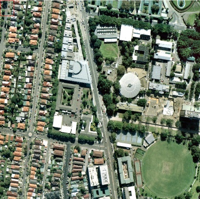 | Figure 1. The study area located in the University of New South Wales campus, Sydney, Australia |
Table 1. Characteristics of image datasets
 |
| |
|
Table 2. Characteristics of LiDAR datasets
 |
| |
|
3. Methodology
To detect building patches, a DTM and a DSM are generated from LiDAR data. After that, nDSM is calculated by subtracting DTM from DSM and then 3D objects are separated by applying a 3m threshold to nDSM. An orthoimage is then generated from the high resolution image using the DSM. The orthorectification of the image is necessary to accurately overlay the image with the reference building database. To detect the candidate building patches, the orthorectified high resolution image is classified utilizing the nDSM and additional bands.
3.1. Image Preparation
Image preparation includes the generation of nDSM, the normalized difference vegetation index (NDVI), training data set and reference data. The nDSM was generated by subtracting the DTM from the DSM as shown in Figure 2(a), (b) and (c). The nDSM represents the absolute heights of non-ground objects, such as buildings and trees, above the ground. Finally, a height threshold of 3m was applied to the nDSM to eliminating other objects such as cars to ensure that they are not included in the final classified image. After detection of the objects with high elevation, buildings should be separated from trees. The NDVI is the most useful factor to extract trees.The NDVI values were generated by using the red image and the LiDAR reflectance values, since the radiation emitted by the LiDARs is in the IR wavelengthsas shown in Figure 2 (d).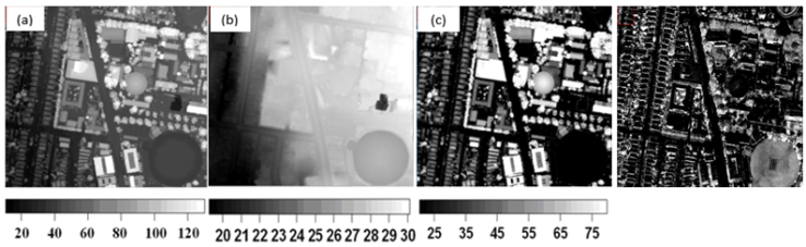 | Figure 2. (a) DSM generated from the original LiDAR point cloud, (b) DTM generated by filtering of LiDAR data, (c) nDSM generated by subtracting the DTM from the DSM and (d) NDVI |
The objective of training datasets is to assemble a set of statistics that describe the spectral response patterns for each land cover type to be classified in the image [16]. The positions of the polygons were selected carefully to be representative and to capture changes in the spectral variability of each class. Each sample was then converted into a vector representing the attributes or features. The training data for their region consists of 7153, 2371, 1508 and 519 training pixels for buildings, trees areas, roads and grass respectively for each band of the input data. Samples of these signatures are shown in Figure 3 (a), (b), (c) and (d).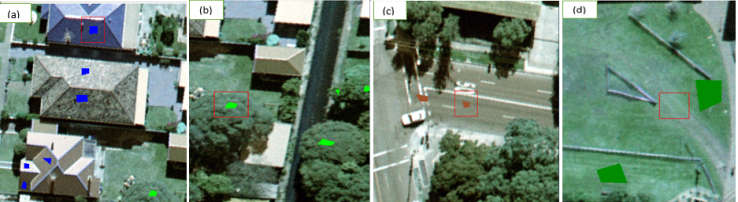 | Figure 3. Sample of signature (a) buildings signatures, (b) trees signatures, (c) roads signatures and (d) grass signatures |
The training datasets along with the orthophoto (red, green and blue bands), the NDVI, DSM, DTM, nDSM and intensity image have been applied as input data for SVMs and ANNs classifier. Reference data were generated by digitizing buildings, trees, roads and grass in the orthophotos. All recognizable features independent of their size were digitizedas shown in Figure 4.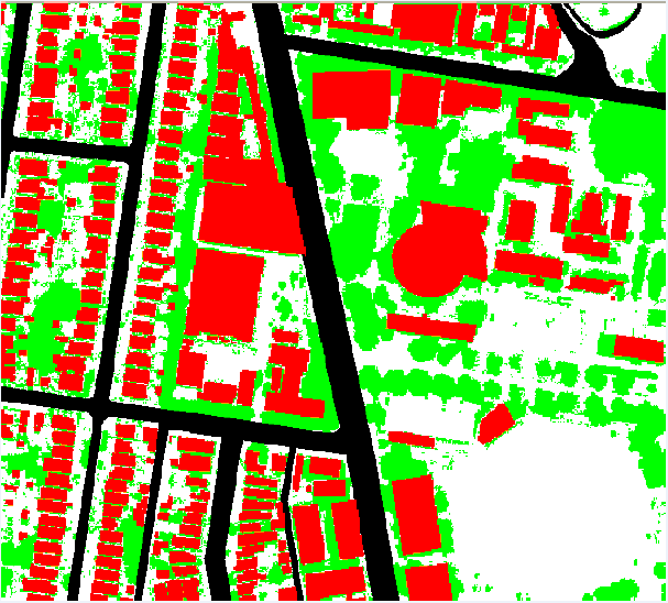 | Figure 4. Reference Data. The red, green, black and white color indicate for buildings, trees, roads and Grass, respectively |
3.2. Image Classification
Two classification techniques have been applied for classifications which include: SVMs and ANNs. The results were then combined using serial, parallel and hybrid combination systems.
3.2.1. SVMs
SVMs are binary classifier delineate two classes by fitting an optimal separating hyperplane to the training data in the multidimensional feature space to maximize the margin between them. The maximum distance between training data of both classes maximizing the margin distance provides some reinforcement so that future data points can be classified with more confidence. Given a training dataset of n points of the form (x1, y1)… (xn, yn) where the yi are either 1 or −1, indicating the class to which the point xi belongs. Each xi is a p-dimensional real vector. The objective is to find the "maximum-margin hyperplane" that divides the group of points xi for which yi = 1 from the group of points for which yi = −1, so that the distance between the hyperplane and the nearest point xi is maximized. Any hyperplane can be written as a set of points x satisfyingin equation (1): | (1) |
In Figure 5, w is an n-dimensional vector perpendicular to the hyperplane, and b is the distance of the closest point on the hyperplane to the origin. Two parallel hyperplanes are applied to separate the two classes of data, so that the distance between them is as large as possible. The region bounded by these two hyperplanes is referred to as "margin", and the maximum-margin hyperplane is the hyperplane that lies halfway between them. With a normalized or standardized dataset, these hyperplanes can be described by the equations (2) and (3). The distance between these two hyperplanes is  . These constraints state that each data point must lie on the correct side of the margin. This can be rewritten as equation (4):
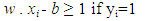 | (2) |
 | (3) |
 | (4) |
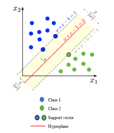 | Figure 5. Optimum separation plane |
To project the data from input space into feature space kernel functions such as Gaussian Radius Basis Function (RBF), Linear, Polynomial and Sigmoid (Quadratic) can be applied. The RBF kernel has proved to be effective with reasonable processing times [17]. Two parameters have to be specified in order to use the RBF kernels: (1) the penalty parameter, C, that controls the trade-off between the maximization of the margin between the training data vectors and the decision boundary plus the penalization of training errors; (2) the width of the kernel function, γ. The output of SVMs represents the distances of each pixel to the optimal separating hyperplane, referred to as rule images. All positive (+1) and negative (-1) votes for a specific class are summed and the final class membership of a certain pixel is derived by a simple majority voting.
3.2.2. ANNs
An ANN is a form of artificial intelligence that imitates some functions of the human brain. All neurons on a given layers are linked by weighted connections to all neurons on the previous and subsequent layers. An ANN consists of a series of layers, each containing a set of processing units (neurons). During the training phase, the ANNs learn about the regularities present in the training data, and based on these regularities, ANNs construct rules that can be extended to the unknown data [18]. A well-trained network is capable of classifying highly complex data. There are several ANNs algorithms that can be used to classify remotely sensed images which include: multi-layer perceptron (MLP), fuzzy artmap classification, self-organized feature map (SOM) and radial basis function network (RBFN). MLP, the most widely used type of ANNs, has been applied in this research. It is a feed-forward ANNs model that maps input data sets onto a set of appropriate outputs. A perceptron element consists of a single node which receives weighted inputs and thresholds the results according to a rule. The perceptron is able to classify linearly separable data, but is unable to handle non-linear data. A neural network consists of a number of interconnected nodes (equivalent to biological neurons). Each node is a simple processing element that responds to the weighted inputs it receives from other nodes. The arrangement of the nodes is referred to as the network architecture as shown in Figure 6. The MLP can separate data that are non-linear because it is `multi-layer’, and it generally consists of three (or more) types of layers. It has been assumed that the number of layers in a network refers to the number of layers of nodes and not to the number of layers of weights. 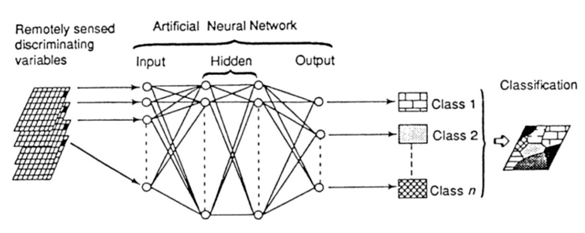 | Figure 6. MLP with back-propagation |
The first type of layer is the input layer, where the nodes are the elements of a feature vector. This vector might consist of the wavebands of a data set, the texture of the image or other more complex parameters. The second type of layer is the internal or `hidden’ layer since it does not contain output units. There are no rules, but theory shows that one hidden layer can represent any Boolean function. An increase in the number of hidden layers enables the network to learn more complex problems, but the capacity to generalize is reduced and there is an associated increase in training time suggests that if a second hidden layer is used, the maximum number of nodes in the second hidden layer should be three times the number in the first hidden layer. The third type of layer is the output layer and this presents the output data which represent in image classification, the number of nodes in the output layer is equal to the classes in the classification and following layers by connections [19]. Back-propagation for training the network can be expressed mathematically as shown in equation (5). w refers to the vector of weights, x is the vector of inputs, b is the bias and φ is the activation function. | (5) |
3.3. Multiple Classifier Systems (MCS)
MCS are based on the combination of different classifier algorithms, so the individual advantages of each method can be combined. Three forms of MCS have been tested and compared which includes: 1) serial combination, 2) Parallel combination, and 3) Hierarchical (hybrid) combination [20].
3.3.1. Serial Combination
The classification result generated by a classifier is used as the input into the next classifier until a result is obtained through the final classifier in the chain. In this research the results from SVMs have been applied as input to ANNs as shown in Figure 7.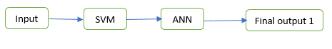 | Figure 7. Serial combination |
3.3.2. Parallel Combination
Multiple classifiers are designed independently and their outputs are combined according to certain strategies. In this research we combine the classification result for SVMs and ANNs using the maximum rule as shown in Figure 8.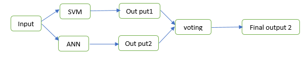 | Figure 8. Parallel combination |
3.3.3. Hierarchical (Hybrid) Combination
Hybrid systems are normally used to combine both the serial and parallel MCS. The most common used hybrid systems are: Maximum Rule (MR), Dempster-Shafer Theory (DST), Weighted Sum (WS) and Fuzzy Majority Voting (FMV). The maximum rule (MR) has prooved to be effective in combining high dimensional data with high accuracy as well as low processing time and has been applied for combining both the serial and parallel results as shown in Figure 9. 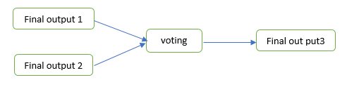 | Figure 9. Hierarchical (hybrid) combination |
MR is a simple method for combining probabilities provided by multiple classifiers. It interprets each class membership as a vote for one of the k classes. For each individual classifier, the class that receives the highest-class membership is taken as the class label for that classifier. After that, the class labels from the N classifiers are compared again and the class that receives the highest class membership is taken as the final classification as in equation (6) is the class membership of a pixel to belong to a class Ck given by classifier fi, and PMR is the probability based on MR [12].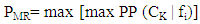 | (6) |
4. Results and Discussion
To perform the SVMs classification, pairs of (C, γ) were tested and the one with the best cross-validation accuracy was selected. First we applied a coarse grid with ranges of values of [0.001, 0.01, 1,……, 10 000] for both C and γ. Then we applied a finer grid search in the neighbourhood of the best C and γ, obtained from the coarse grid, with ranges of values [(C or γ)-10, (C or γ) +10] and with interval of 0.01 to obtain a better cross-validation. The obtained values are 0.111 and 100 for gamma and penalty parameters respectively. Once C and γ have been specified, they were used with the entire training set, to construct the optimal hyperplane. The out put from the SVMs classifier are probabilities in the range of 0 to 1, where 0.0 expresses absolute improbability and 1.0 expresses a complete assignment to a class. A typical view of the SVMs output, the decision values of each pixel for each class, is shown in Figure 10. The membership values from all the land covers were compared and the class with the highest membership value was assigned to the pixel label to obtain the final SVMs classification as shown in Figure 13(b).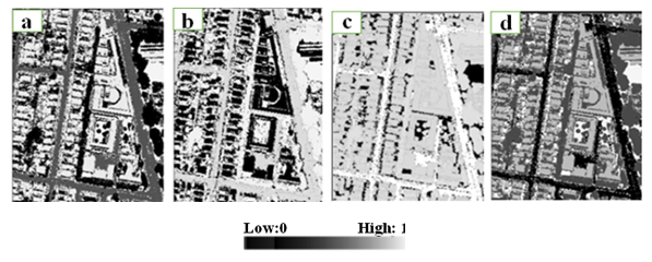 | Figure 10. Atypical view of membership values of the SVMs output: (a) Buildings, (b) Trees, (c) Roads, and (d) Grass classes |
 | Figure 11. Atypical view of membership values of the ANNs output: (a) Buildings, (b) Trees, (c) Roads and (d) Grass classes |
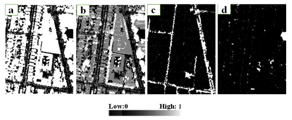
 | Figure 12. Atypical view of membership values of the hybrid system: (a) Buildings, (b) Trees, (c) Roads and (d) Grass classes |
To perform the ANNs classification, the structure of the MLP model was as follows: the numbers of input, hidden and output layer neurons were 8, 1 and 8 respectively; training threshold contribution=0.90; training rate=0.200; training RMS exit criteria 0.10 and number of training iteration=1000. A typical view of the ANNs output, the decision values of each pixel for each class, is shown in figure 11. The membership values from all the land covers were compared and the class with the highest membership value was assigned to the pixel label to obtain the final ANNs classification as shown in Figure 13(c). The probability values (images) obtained from SVMs and ANNs were then combined in serial, parallel and hybrid forms in order to estimate the combined probabilities. A typical view of membership values of the hybrid system is given in figure 12. Once again, the membership values from all the land covers were compared and the class with the highest membership value was assigned to the pixel label. Typical views of the serial, parallel and hybrid systems classification results are shown in Figure 13(d), (e) and (f). 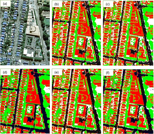 | Figure 13. a typical view of the classification results. (a) orthophoto, (b) SVMs classified image, (c) ANNs classified image, (d) serial combination classified image, (e) parallel combination classified image, (f) hybrid (MR) classified image. The colors indicate the different classes: Red for buildings, Green for trees, Black stands for roads and White for Grass |
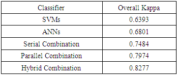
4.1. Overall Kappa
The results for SVMs, ANNs, serial combination, parallel combinations and hybrid system have been compared with the reference data. The overall Kappa of single classifiers aw well as hybrid systems are summarized in Table 3.Table 3. Overall Kappa of single classifiers and hybrid systems
 |
| |
|
The overall kappa for individual classifiers was 0.6393 and 0.6801 for SVMs and ANNs respectively. The hybrid system has performed the best with 0.8277 overall kappa followed by parallel combination and serial combination with 0.7974 and 0.7484 overall kappa, respectively.A closer examination of the SVMs and ANNs results reveals that the kappa coefficient is relatively low, indicating these methods are unsatisfactory for classifying remotely sensed images if they are not incorporated into a combination system. The improvement in overall Kappa achieved by the three combination methods compared with the best individual classifier are 0.0683, 0.1173 and 0.1476 for serial, parallel and hybrid systems respectively.
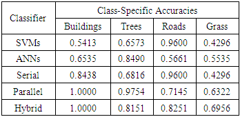
4.2. Class Accuracy
The kappa index of agreement (KIA) is statistical measure and has been adapted for class-accuracy assessment in this research. Class accuracies of single classifiers as well as hybrid systems are summarized in Table 4. For buildings, the hybrid and parallel systems have achieved the best class accuracies with 1.000 KIA followed by serial combination, ANNs and SVMs with 0.8438, 0.6535 and 0.5413 KIA respectively. For trees, the parallel combination achieved the best rsults with 0.9754 KIA followed by ANNs, hybrid combination, serial combination and SVMs with 0.8490, 0.8151, 0.6816 and 0.6573 KIA respectively. For roads, SVMs and serial combination achieved the best results with 0.9600 KIA followed by the hybrid system, parallel system and ANNs with 0.8251, 0.7145 and 0.5661 KIA respectively. For grass, the hybrid combination achieved the best results with 0.6956 KIA followed by the parallel combination and ANNs with 0.6322 and 0.5535 respectively. SVMs and serial Combination have performed the worst with the same KIA, 0.4296.Table 4. Class-Specific Accuracies of single classifiers and hybrid systems
 |
| |
|
An assessment of the KIA confirms that the hybrid system performed the best in most cases as shown in table 4. Most of the class-accuracies are improved by the hybrid system. Whereas the application of SVMs and ANNs resulted in average KIA of 0.64705 and 0.62455 respectively, the application of the combination systems resulted in average KIA of 0.72875, 0.779875 and 0.76745 for serial, parallel and hybrid systems respectively. Another advantage of the hybrid systems is that the achieved errors are less variable. Whereas the application of SVMs and ANNs resulted in standard deviation of 0.1978 and 0.1182, for KIA, the application of the combination systems resulted in average KIA of 0.1990, 0.1601 and 0.1086 for serial, parallel and hybrid systems respectively.Finally, it is worth noting that the classification accuracy for the land cover classes of trees and roads using the hybrid system is lower compared to those using Parallel and Serial techniques. Under such an observation, if a particular class is very important, different combination techniques have to be tested first to select the best combination method for that class.
5. Conclusions
In this paper, automatic building extraction procedure within classification approaches has been applied. Aerial image with spatial resolution 9cm, LiDAR data and other ancillary data have been applied as input data for different classification approaches. SVMs and ANNs classifiers were tested and compared to classify buildings, trees, roads and grass. The results show that the ANNs method has achieved an overall kappa of 0.6801, compared with 0.6393 that was obtained from the SVMs method. The improvements of overall kappa that were obtained by combining SVMs and ANNs classifiers have been reported. Hybrid Combination performed the best with 0.8277 overall kappa followed by parallel combination and serial combination with 0.7974 and 0.7484 overall kappa respectively.
References
| [1] | Lee, D. S., Shan, J. and Bethel, J. S., 2003. Class-Guided Building Extraction from IKONOS imagery, Photogrammetric Engineering and Remote Sensing, 69(2), pp.143-150. |
| [2] | Jin, X. and Davis, C. H., 2005. Automated Building Extraction from High Resolution Satellite Imagery in Urban Areas Using Structural, Contextual, and Spectral Information, Eurasip journal on applied signal processing. |
| [3] | Zahra Lari and Hamid Ebadi, 2007. Automated Building Extraction from High-Resolution Satellite Imagery Using Spectral and Structural Information Based on Artificial Neural Networks, ISPRS Journal of Photogrammetry and Remote Sensing. |
| [4] | Omo-Irabor, and O.O, 2016. A Comparative Study of Image Classification Algorithms for Landscape Assessment of the Niger Delta Region, Journal of Geographic Information System, 8, 163-170. |
| [5] | L. Zhu, H. Shimamura, K. Tachibana, Y. Li and P. Gong, 2008. Building Change Detection based on Object Extraction In Dense Urban Areas, The International Archives of the Photogrammetry, Remote Sensing and Spatial Information Sciences. Vol. XXXVII. Part B7. |
| [6] | Woosug Cho, Yoon-Seok Jwa, Hwi-Jeong Chang and Sung-Hun Lee, 2004. Pseudo-Grid Based Building Extraction Using Airborne LIDAR Data, Int Arch Photogrammetry Remote Sens Spat Inf Sci. |
| [7] | N. Jiang, J.X. Zhang, H.T. Li and X.G. Lin, 2008. Object-oriented building extraction by DSM and very high-resolution orthoimages, ISPRS Journal of Photogrammetry and Remote Sensing, Commission III, WG III/4. |
| [8] | Zheng Wang, 2000. Building Extraction and Reconstruction from LiDAR Data, International Archives of Photogrammetry and Remote Sensing. Vol. XXXIII, Part B3. |
| [9] | D. Koc San and M. Turker, 2010. Building Extraction from High Resolution Satellite Images Using Hough Transform, International Archives of the Photogrammetry, Remote Sensing and Spatial Information Science, Volume XXXVIII, Part 8. |
| [10] | TxominHermosilla, Luis A. Ruiz, Jorge A. Recio and Javier Estornell, 2011. Evaluation of Automatic Building Detection Approaches Combining High Resolution Images and LiDAR Data, Remote Sens., Volume 3, PP. 1067-1283. |
| [11] | Yan Li, Lin Zhu and Hideki Shimamura, 2008. Integrated Method of Building Extraction from Digital Surface Model and Imagery, The International Archives of the Photogrammetry, Remote Sensing and Spatial Information Sciences. Vol. XXXVII. Part B3b. |
| [12] | Kazuo Oda, Tadashi Takano, Takeshi Doihara And Ryosuke Shibasa, 2015. Automatic Building Extraction and 3-D City Modeling from LiDAR Data based on Hough Transformation, Commission III, PS WG III/3. |
| [13] | Pakorn Watanachaturaporn, Manoj K. Arora and Pramod K. Varshney, 2008. Multisource Classification Using Support Vector Machines: An Empirical Comparison with Decision Tree and Neural Network Classifiers, American Society Of Photogrammetry And Remote Sensing, 74(2), pp.239–246. |
| [14] | M. Salah, J.C. Trinder, A. Shaker, M. Hamed and A. Elsagheer, 2010. Integrating Multiple Classifiers With Fuzzy Majority Voting For Improved Land Cover Classification, The International Archives of the Photogrammetry, Remote Sensing and Spatial Information Sciences, Vol. XXXVIII, Part 3A. |
| [15] | M.salah, 2014. Combined Pixel Based and Object -Oriented Support Vector Machines Using Bayesian Probability Theory, ISPRS Annuals of The Photogrammetry, Remote sensing and Spatial information sciences. |
| [16] | Lillesand, T. and R. Kiefer, 2004. Remote Sensing and Image Interpretation. Fourth Edition, John Willey & Sons, Inc., New York. |
| [17] | M.Salah, 2017. A Survey of Modern Classification Techniques in Remote Sensing for Improved Image Classification, Journal of Geomatics Vol 11 No. 1. |
| [18] | Foody and G.M., 1999. Image classification with A neural network: From completely crisp to fully-fuzzy situations, In P.M. Atkinson and N.J. Tate (eds), Advances in Remote Sensing and GIS analysis, Chichester: Wiley & Son. |
| [19] | P. M. Atkinson and A. R. L. Tatnal, 2010. Introduction Neural networks in remote sensing, International Journal of Remote Sensing, 18(4), pp. 699-709. |
| [20] | Michał Woz´niaka, Manuel Graña and Emilio Corchadoc. 2014. A survey of multiple classifier systems as hybrid systems. Information Fusion, 16: 3–17. |
| [21] | ENVI Manual. Version 5.3. |
| [22] | L3 Harris Geospatial Solution |

 Abstract
 Reference
 Full-Text PDF
 Full-text HTML