Abdallah A. Saad, Mona S. El-Sayed
Surveying Engineering Department, Faculty of Engineering- Shoubra, Benha University, Egypt
Correspondence to: Mona S. El-Sayed, Surveying Engineering Department, Faculty of Engineering- Shoubra, Benha University, Egypt.
| Email: |  |
Copyright © 2019 The Author(s). Published by Scientific & Academic Publishing.
This work is licensed under the Creative Commons Attribution International License (CC BY).
http://creativecommons.org/licenses/by/4.0/

Abstract
Nowadays, precise geoid is importantly and urgently needed in Egypt for many applications. For that reason and for the first time, a lot of terrestrial gravity data are collected as gravity values, gravity anomalies, deflection components, and GPS leveling undulations. These data are collected from governmental agencies, petroleum companies, and research institutes and centers. The collected data covers a large area of the Egyptian territory, but they have been taken with different references, strategies, and methodologies. To get use of those heterogeneous multisource data, they should be verified, investigated, filtered, and modified on scientific bases. In this research, some methods of gravity data verification and investigation are proposed. Data verification through undulation differences, undulation rate of change, and undulation acceleration are introduced. 134 observed GPS leveling stations along the River Nile are verified and the odd values are modified. EGM2008 is used against the observed undulations to help in explaining the proposed ideas in this research.
Keywords:
Geoid Undulation, EGM2008, GPS/Levelling, Rate of Change, Undulation Acceleration
Cite this paper: Abdallah A. Saad, Mona S. El-Sayed, Proposals for Evaluating the Observed Gravity Field Data, American Journal of Geographic Information System, Vol. 8 No. 4, 2019, pp. 191-198. doi: 10.5923/j.ajgis.20190804.03.
1. Introduction
It is accepted all over the world that a reference ellipsoid (geodetic datum) is defined to geometrically represent the earth. The adopted reference ellipsoid has uniform gravity field (normal) approximating the actual (natural) one. The actual gravity field of the earth could be divided into a computed uniform ellipsoidal part and the deviations of the actual from the normal gravity field. Those deviations could be gravity anomalies, deflection angles, and geoid undulations, which are the gravity field elements [1]. A large number of Global Geo-Potential Models (GGMs) have been released and used in geoid modeling all over the world. A basic utilization of GGMs is to represent the long wavelength component of the earth gravitational field in obtaining geoid undulations [2]. Gravity field can be modeled using suitable observations and its elements are obtained by interpolating the obtained model wherever they are needed. So before using the gravity field observations, they have to be subjected to verification, investigation, and filtering processes [3]. Nowadays, the gravity field elements can be determined from satellite missions. In its turn, the satellite gravity mission’s results should be assessed against verified (reliable) terrestrial observations. Most of the work done in this field depended on the full values of the gravity field elements [4]. This produces large values of the obtained mean and RMSE while making assessment (comparison) process [5]. In this research, other styles of assessments are proposed. The data which will be examined here is observed undulations and their corresponding undulations from EGM2008, full values of undulations will be examined against each other. The observed undulations will be converted into differences between every two successive undulations. EGM2008 undulations will also be converted into corresponding difference. Then those successive differences from both groups will be compared to each other. It is expected that the resulted differences will be smaller and smoother than the case of using full undulations in the comparison process. Datum shifts between the two groups (sources) will be excluded from the comparison. Undulation rate of change is introduced to make the comparison between two sources of data more smooth. Undulation rate of change is obtained by dividing the successive difference over the corresponding horizontal distance and its unit will be (cm/km). Undulation acceleration is also introduced to assure if the gravity data contains odd values or not. Undulation acceleration is obtained by dividing the difference between the successive rates of change over the corresponding horizontal distance once more, its unit will be (cm/km2). The proposed ideas in this research will be implemented through 134 observed undulations and their corresponding values from EGM2008 as the best global model in resolution and accuracy. As a spherical harmonic model of the Earth’s gravitational potential, the EGM2008 is established through a least squares combination of the -GRACE03S gravitational model and its associated error covariance matrix. EGM2008 is complete to degree and order 2159, and contains additional coefficients up to degree 2190 and order 2159 [6]. In addition, it applies the gravitational information that obtained from a global set of area-mean free-air gravity anomalies. It is defined on a 5 arc-minute equiangular grid which is formed by merging terrestrial, altimetry-derived, and airborne gravity data. Over areas that lack of the high resolution gravitational data, the spectral content is completed with gravitational information gathered from the topography. In contrast, the availability of the high quality resolution gravity data, the differences between EGM2008 geoid undulations and the values obtained from the /Leveling measurements within the order of ±5 to ± [7]. Such a fact designates that EGM2008 can be applied as a current detailed regional geoid model. Over EGM96, EGM2008 represents improvement by a factor of six in resolution, and by factors of three to six in accuracy, depending on gravitational quantity and geographic area. EGM2008 represents a milestone and a new example in global gravity field modeling, by demonstrating for the first time ever, that given accurate and detailed gravimetric data, a single global model may satisfy the requirements of a very wide range of applications [8]. EGM2008 have been evaluated in different places of the world by several authors [9], [10], [11].
2. Data Used (Observed Undulations – EGM2008 Model)
The used data covers longitudinally from Assiut (Lat. 27° N) to Damietta (Lat. 31° N) along the Nile River. Fixed stations were established every about 5 km apart, covering total distance of about 600 km and the number of those fixed stations are 134, Figure (1).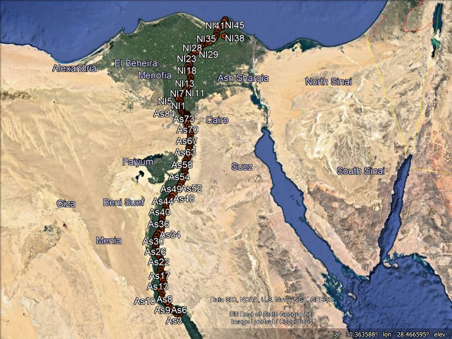 | Figure (1). The available points in the study area |
The geodetic coordinates, referenced to WGS84, of the 134 stations are obtained using GPS observations. Dual frequency GPS receivers are used. Those stations are tied to the nearest stations of the National Agricultural Cadastral Network (NACN) as reference stations. The orthometric heights of the fixed points are obtained by spirit leveling starting from the nearest bench marks of the ministry of irrigation. The mentioned available geodetic dataset, 134 GPS levelling stations have been observed by the Survey Research Institute (SRI) in several surveying sessions. Thus, the geoid undulations at the 134 fixed stations are obtained. The geoid undulations of the 134 stations are extracted also from EGM2008.
3. Methodology and Results
The observed geoid undulations at the fixed stations are obtained from the well-known relation: | (1) |
Where N is the geoid undulation, h is the ellipsoidal height obtained from GPS and H is the orthometric height obtained by spirit leveling.Using the latitude and the longitude of the observed stations, the corresponding geoid undulation values from EGM2008 are obtained from the website http//icgem.gfz-postdam.de/ICGEM/ICGEM.html. So the data will be manipulated are the observed geoid undulations at the 134 stations and their corresponding values from EGM2008. The computations of this research will be run to serve two main purposes;• Data verification to find out the odd values if they exist • Modification of (not to be excluded) the odd values from the observed data file.In the next statistics of the research, the mean and RMSE will be computed from the absolute values of the differences.
3.1. Verification and Finding out of the Odd Observed Undulations
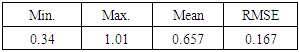
Verification and finding out of the odd observed undulations have been done through the following steps;Step 1: Observed undulations against EGM2008 undulationsThe differences between the observed undulations and their corresponding values from EGM2008 are computed. Most of the researches use these differences in assessing such a field. min, max, mean, and RMSE for those differences are obtained, Table (1). Figure (2) illustrates the observed against EGM2008 undulations along 134 data points. 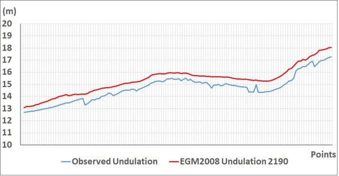 | Figure (2). Observed against EGM2008 undulations along 134 data points |
The figure shows almost a trend shift between the observed and EGM2008 undulations except at the points which do not show harmony among the observed undulations. EGM2008 undulations show consistency along the line of data points. It has to be mentioned here that the gravity field is continuous and it changes geographically in harmony not in a sudden change. Table (1). Statistics of the differences between the observed and EGM2008 undulations (m)
 |
| |
|
The mean of the differences between the observed undulations and their EGM2008 corresponding values is 65.7 cm with 16.7 cm RMSE which refers to the nature of the undulation sources. The resolution of EGM2008 and the absence of terrestrial data of Egypt in the model is to be considered. The reliability of the GPS heights and the orthometric heights while making GPS levelling should also be investigated. The values in the table indicate also that the differences are not consistent or not in good harmony and there are odd values (differences). The GPS work had fixed solutions and the base stations were NACN stations which make the GPS solutions are trustable. Meanwhile the orthometric heights depended on the Bench Marks of the Ministry of Irrigation whereas they suffer lake of maintenance. So to clear the odd observed undulations and to overcome the disturbed shift between the two surfaces, the comparison between the two surfaces is preferred to run through the corresponding differences (not on the full values) from the observations and EGM2008 as in the next steps. So investigations can be done after changing the data from the same source into differences, which makes highlighting the odd values clearer and they can be corrected. The corrected differences can be returned back again to absolute values by using one trustable value. Step 2: The differences between every two successive values from the observed undulationsThe differences between every two successive values in the observed data file are computed as follows: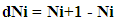 | (2) |
min, max, mean and RMSE of these differences are obtained, Table (2) and Figure (3).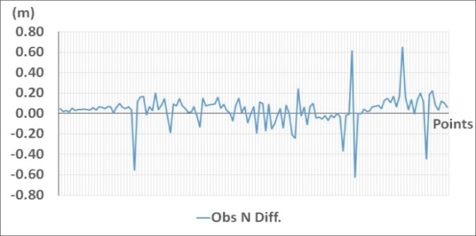 | Figure (3). Successive differences for the observed undulations |
Although the distances between every two successive stations are nearly equal, the differences between every two successive observed undulations do not show harmony (consistency) along the data points. Large values relative to the most others are clear.Table (2). Statistics for the differences of every two successive observed undulations (m)
 |
| |
|
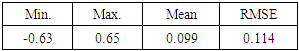
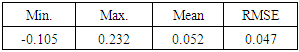
The values of min, max, RMSE with the mean assures the existence of odd differences in the observation file. The range of the observed differences is 1.28 m which makes the RMSEs larger than the mean value. Step 3: The differences between every two successive values from EGM2008.The computations in step 2 are done for the undulation values of EGM2008, Table (3) and Figure (4).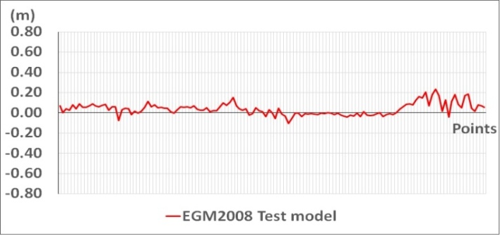 | Figure (4). Successive differences for EGM2008 undulations |
Unlike the case of observed data, the successive EGM2008 undulation differences show harmony in their changing along the data line. EGM2008 undulation may have a resolution problem but they may introduce a trend without mistakes. Table (3). Statistics of the differences of every two successive undulations of EGM2008 (m)
 |
| |
|
The table assures that the case of EGM2008 differences is obviously different from the case of the observed differences where the range is 33 cm and RMSE is not larger than the mean. This indicates that EGM2008 values are better in consistency and in harmony.Step 4: Observed successive undulation differences against EGM2008 successive undulation differences The differences between the differences in step 2 and their corresponding differences in step 3 are computed, drawn in Figure (5) and their min, max, mean and RMSE are in Table (4). This step is done to clarify and assure the stations where odd values are existing.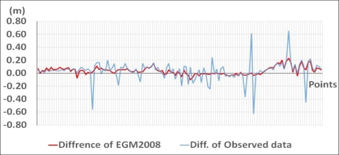 | Figure (5). Successive observed undulation differences against their corresponding EGM2008 values |
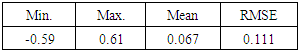
The figure depicts a general agreement except at the points which are inconsistent among the observed differences.Table (4). Statistics of the differences between observed differences and EGM2008 differences (m)
 |
| |
|
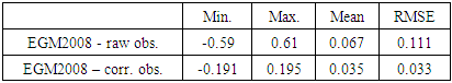
The large range (1.2 m) and RMSE larger than the mean indicate again that the differences in the observed file have odd values. Here the mean of the differences between observed and EGM2008 differences (6.7 cm) with (11.1 cm) RMSE is obviously smaller than the case of differences of the full undulation values in Table (1) with mean (65.7 cm) and RMSE (16.7 cm). It means that considering the undulation differences is much useful than using the undulation values themselves. It means also that extracting a trend shift then relating those differences to one reliable undulation value will help in obtaining more trustable gravity field. Step 5: Rate of change for both observed and EGM2008 undulationsThe obtained differences in steps 2 and 3 are divided over their corresponding horizontal distances, i.e. the horizontal distance between the two successive bench marks (i+1) and (i) to obtain the rate of change of the geoid undulation w.r.t the corresponding horizontal distance. These values are expressed in cm/km. The successive differences in the last step may not well reveal the consistency in the field because the inequality of the distances among the data points. So, the rate of undulation change as (cm/km) is introduced to be more stable indicator for the consistency (harmony) of the gravity field over certain path or area.Undulation rate of change = (N(i+1) – N(i)) / D(i+1), (i)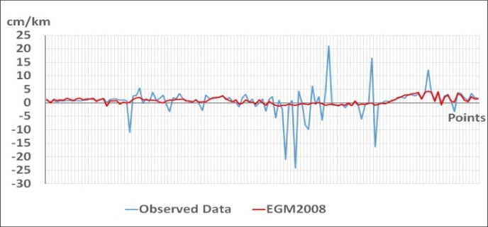 | Figure (6). Undulation rate of change from observed data against the EGM2008 corresponding values |
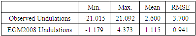
Again the values of undulation rate of change in the case of EGM2008 show harmony unlike the case of the observed data which contains odd values. Recalling that the gravity field does not change suddenly but it is a consistent field. This is clear in EGM2008 data and is not in the observed data. Table (5). Statistics of rate of change of observed and EGM2008 undulations (cm/km)
 |
| |
|
The large range (42.1 cm) in the observation file against the small range (5.55 cm) in the EGM2008 file assures the presence of mistakes in the observation file again. Step 6: Undulation acceleration for the observed and EGM2008 undulations.To obtain more smoothed image of a gravity field, the undulation acceleration is proposed. Undulation acceleration is obtained by dividing the undulation rate of change by the corresponding horizontal distance once more and its unit will be cm/km2.  | (3) |
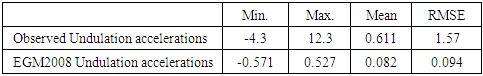
Undulation accelerations are computed for both observations and EGM2008 and illustrated in Figure (7) and the statistics are in Table (6).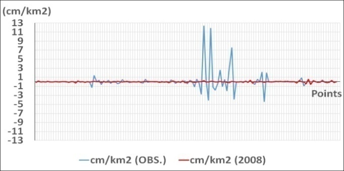 | Figure (7). Observed undulation accelerations against their EGM2008 corresponding values |
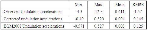
Table (6). Statistics of undulation accelerations for observed data and EGM2008 (cm/km2)
 |
| |
|
The values of the undulation acceleration in the case of EGM2008 almost tend to (approaching) zero which indicates harmony (consistency) in the gravity field in the considered area. The corresponding values of the observed data are not alike and they suffer inconsistency because of the existence of odd values.
3.2. Treating the Odd Values of Undulations in the Observed Data File
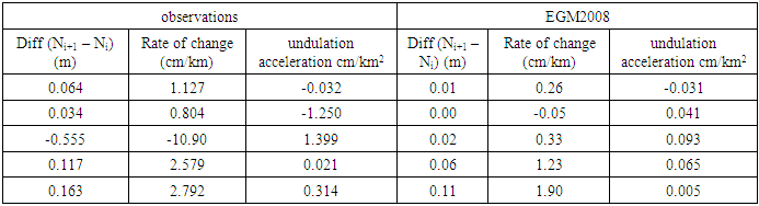
Odd values of undulations are defined after revising the observed undulation file in the light of:1. Comparing every observed undulation value with the preceding and succeeding values.2. Comparing every observed undulation value with its corresponding EGM2008 value.3. Comparing every observed difference value, (difference between every two successive undulations), with the preceding and succeeding values.4. Comparing every observed successive difference value with its corresponding value from EGM2008.5. Comparing every observed undulation rate of change with the preceding and succeeding values.6. Comparing every observed undulation rate of change with its corresponding value from EGM2008.7. Comparing every observed undulation acceleration with the preceding and succeeding values.8. Comparing every observed undulation acceleration with its corresponding value from EGM2008.Nineteen difference values out of 133 are considered to be odd according to the explained criteria. An example of those cases is shown in Table (7).Table (7). An example of defining an odd value as an application of the above mentioned comparisons
 |
| |
|
The values in red color are odd w.r.t the preceding and the succeeding values and also w.r.t the corresponding value from EGM2008.Therefore, the following scenarios could be proposed:1. Excluding the odd values if they are not necessarily needed2. Taking the corresponding value from EGM2008 instead 3. Computing new value based on the linear interpolation from the two preceding and succeeding values. Recalling that the interpolation will be over distance does not exceed 10 km; | (4) |
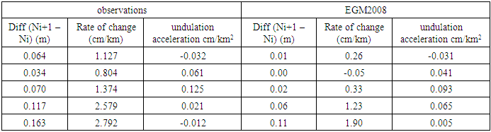
Where:Ni is the interpolated undulation value at station iNi-1 is the observed preceding undulation value to station iNi+1 is the observed succeeding undulation value to station iD1 is the horizontal distance between station (i-1) and station (i+1) D2 is the horizontal distance between station (i-1) and station (i)The third scenario is adopted in this research and the odd observed undulations are modified, Table (8). Figure (8) illustrates the modified observed values after applying the proposed modification. Table (8). The modification of the odd values shown in table (7)
 |
| |
|
The values in red color are the corrected ones and it is clear that they became matching (consistent) with their succeeding and preceding values and also w.r.t the corresponding values of EGM2008.The following figures show the above studied cases after applying the proposed corrections for the observations; 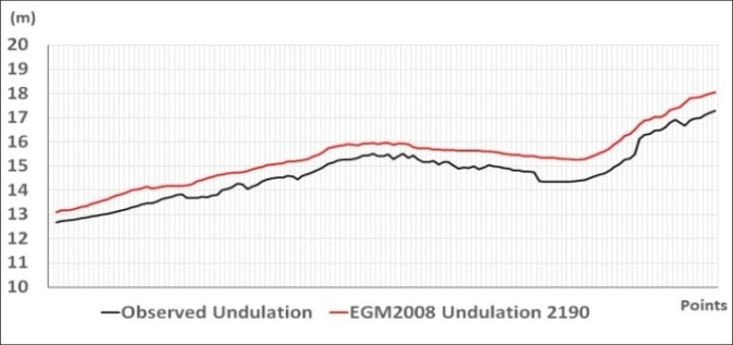 | Figure (8). Corrected observed undulations against EGM2008 undulations |
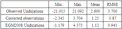
Table (9). Statistics of the differences between the observed and EGM2008 undulations (m)
 |
| |
|
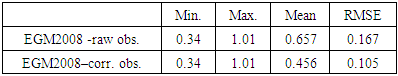
The figure shows that the observed undulations became more smother w.r.t EGM2008 undulations after correcting the odd observed values.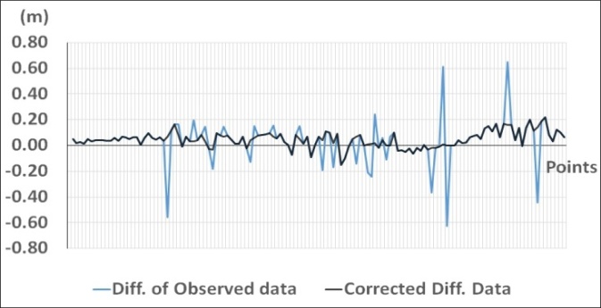 | Figure (9). Corrected observed undulation differences against their corresponding raw observed undulation differences |
It is clear from the figure the harmony which occurred in the observations after modification. Then the modified file of the observed differences is drawn against the corresponding values from EGM2008, Figure (10), to show that the observed differences became closer and similar to the case in EGM2008 without odd values.  | Figure (10). Corrected observed undulation differences against their corresponding EM2008 undulation differences |
Table (10). Statistics of the differences between observed differences and EGM2008 differences (m)
 |
| |
|
Undulation Rate of change is computed in both cases of modified observation file and EGM2008 and illustrated against each other in Figure (11). The figure shows that the observed rates of change after modification became very close to their EGM2008 corresponding values.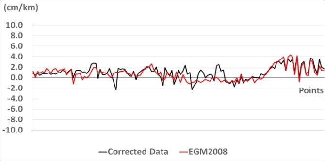 | Figure (11). Corrected observed undulation rates of change against EGM2008 undulation rates of change |
Table (11). Statistics of rates of change of raw observed, corrected observed and EGM2008 undulations (cm/km)
 |
| |
|
The corrected observed rate of change is in better consistency and more closer to that of EGM2008. Finally, undulation acceleration values from both cases are computed and depicted in Figure (12).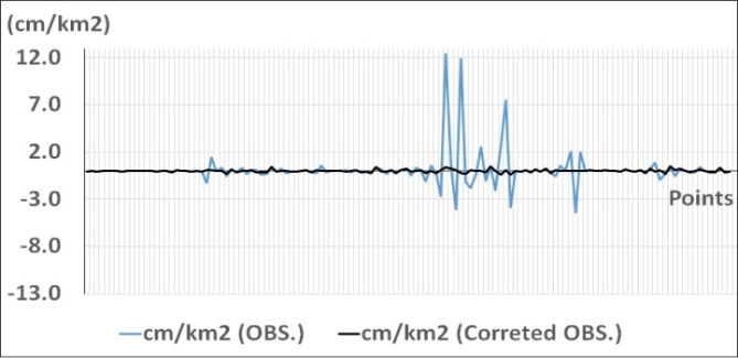 | Figure (12). Corrected observed accelerations against their corresponding values from raw observations |
It is clear in the figure the effect of correcting the observed undulation accelerations and the obtained consistency.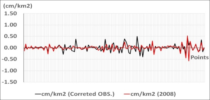 | Figure (13). Corrected observed accelerations against their corresponding EGM2008 values |
Table (12). Statistics of undulation accelerations for raw observed, corrected observed data and EGM2008 (cm/km2)
 |
| |
|
The mean and RMSE of the corrected undulation accelerations have improved and have become very close to those of EGM2008.
4. Conclusions
In Egypt, heterogeneous gravity data (observations) all over the country have been taken by different agencies with different accuracies, references, and strategies. To benefit from all these data to figure the gravity field in Egypt, those data should be examined, investigated, and corrected if needed. The usual way for checking up the observed data is to compare them with their corresponding values from trustable gravity field model. Some ideas are proposed in this research for investigating the gravity data. Those proposals depended on the characteristics of the earth's gravity field. The gravity field is continuous field and it does not generally change suddenly but smoothly. So investigating the observed data as differences besides using the full values is introduced. Undulation rate of change is also introduced to depict the change of the field as (cm/km). it is expected that the introduced rate of change changes smoothly on the local and regional basis. Moreover, the undulation acceleration is proposed in investigating and filtering the observed gravity data. Those proposed ideas are applied on 134 GPS leveling stations have been taken along the River Nile along about 600 km. again, Besides comparing the undulation values as usual, comparing undulation differences is proposed. Undulation rate of change and undulation acceleration are also introduced.The introduced ideas are applied on observed undulations and their corresponding EGM2008 values. In the case of comparing the undulations themselves, the mean (RMSE) of the raw data were 65.7 (16.7) cm and 45.6 (10.5) cm after applying the proposed correction. While in the case of using the undulation differences in the comparison they were 6.7 (11.1) cm for the raw data and 3.5 (3.3) cm for the corrected data. The mean (RMSE) in the case of undulation rate of change of raw data were 2.6 (3.7) cm/km and after correction they were 1.25 (0.87) cm/km. in the case of raw undulation acceleration they were 0.61 (1.57) cm/km2 and 0.004 (0.14) cm/km2. The values of rate of change and undulation acceleration of the corrected data are very close to their corresponding values from EGM2008. Finally and based on the results in the tables and the figures, the proposed ideas of investigating the observed gravity field elements are much smoother than using the full elements themselves. So, they are more powerful in highlighting the consistency of the field. In a developing country like Egypt, it is important to benefit from the observations of the gravity field specially that the high resolution global gravity models do not represent the field in Egypt in good level because of the lake of contribution of the terrestrial data in Egypt into those models. Gravity field data in Egypt are obtained with different references, accuracies, and methodologies. So this research introduces some proposals for investigating, collecting, and correcting those data. Then the collected, unified and corrected data in Egypt and such countries can contribute in improving the global gravity models.
References
| [1] | N.K., Pavlis, S.A., Holmes, S.C., Kenyon, J.K., Factor “An Earth Gravitational Model to Degree 2160: EGM2008”, General Assembly of the European Geosciences Union, Vienna, Austria, 2008. |
| [2] | G., Dawod, H., Mohamed, and S., Ismail “ Evaluation and Adaptation of the EGM2008 Geo-potential Model along the Northern Nile Valley, Egypt: Case Study” Journal of Surveying Engineering, Vol. 136, pp. 36-40 No. 1, http/doi.org 10.1061/(ASCE) SU, 1943-5428.0000002, 2010. |
| [3] | G., Kotsakis “Transforming ellipsoidal heights and geoid undulations between different geodetic reference frames”. Journal of Geodesy, 82: 249-260, 2008. |
| [4] | T., Saari and M., Koivula “Evaluation of GOCE-based Global Models in Finnish Territory”. National Land Survey of Finland. URI: http://hdl.handle.net/10183/224774, 2015. |
| [5] | S., Lee, and C., Kim “Development of regional gravimetric geoid model and comparison with EGM2008 gravity field model over Korea”, Scientific Research and Essay, Vol. 7, No. 3, pp.387-397, 2012. |
| [6] | International Center for Global Gravity Field Models (ICGEM), Available online, http://icgemgfz-potsdam.de/ICGEM/2018. |
| [7] | M., Bilker- Koivula “Assessment of high resolution global gravity field models for geoid modelling in Finland”. Proceeding of the international Symposium on Gravity, Geoid and Height Systems. IAG Symposium, Vol. 141, 2015. |
| [8] | N.K. Pavlis, S.A. Holmes, S.C.Kenyon, and J. K. Factor “The development and evaluation of the earth Gravitational Models 2008 (EGM2008)”, Journal of Geophysics, Vol. 117, 1-38, http:/doi.org/10.1029/2011jb008916, 2012. |
| [9] | J., Huang, and M., Veronneau “Evaluation of the GRACE- Based Global Gravity Models in Canada”. Geodetic Survey Division, CCRS, Natural Resources Canada, Ontario, Canada, 2018. |
| [10] | E., Al-Karagy, M., Doma. and G., Dawod “Towards an accurate discrimination of the local geoid model in Egypt using GPS/leveling data: A case study at Rosetta area”, The International Journal of Innovative Science and Modern Engineering, Vol. 2, No. 11, pp. 10-15, 2014. |
| [11] | A. P., Odera, Y., Fukuda “Evaluation of GOCE-based global gravity field models over Japan after the full mission using free-air gravity anomalies and geoid undulations”. Earth, Planets and Space (2017) 69: 135, http/doi.org/10.1186/s40623-017-0716-1, 2017. |

 Abstract
 Reference
 Full-Text PDF
 Full-text HTML