Fahad S. Alahmadi
Ministry of Environment, Water and Agriculture, Madinah Branch, Saudi Arabia
Correspondence to: Fahad S. Alahmadi, Ministry of Environment, Water and Agriculture, Madinah Branch, Saudi Arabia.
| Email: |  |
Copyright © 2019 The Author(s). Published by Scientific & Academic Publishing.
This work is licensed under the Creative Commons Attribution International License (CC BY).
http://creativecommons.org/licenses/by/4.0/

Abstract
Groundwater as one of the most important global natural resources needs to be quantified and the boundary of aquifers should to be specified for water resources planning and management purposes. Delineation of groundwater aquifers is usually accomplished by geophysical tools and ground penetration radar technology, which are considered as time consuming and relatively expensive. In this study, 1053 groundwater well locations are collected to delineate the aquifer boundaries using spatial clustering techniques in Madinah, Western Kingdom of Saudi Arabia (KSA). The first step in the analysis is assessing the clustering tendency (ACT) using Hopkins statistic and visual assessment of cluster tendency (VAT) approach, both methods showed that the data is spatially random (clusterable), Three spatial density-based clustering (SDBC) approaches are used, which are density-based spatial clustering of applications with noise (DBSCAN), hierarchical density-based spatial clustering of applications with noise (HDBSCAN) and ordering points to identify the clustering structure (OPTICS). Two input parameters are required, which are the minimum numbers of points per cluster (MinPts), and the search radius distance (ε). It was found that the optimum value for MinPts is about 10 and the corresponding (ε) value is computed using K-nearest neighbor distance plot (KNN) and it was found that (ε) is about 1,000 m. The number of clusters produced by the three methods DBSCAN, HDBSCAN, and OPTICS are 6, 19, and 7, respectively, while the number of noise are 89, 313, and 95, respectively. It can be seen that HDBSCAN methods produced higher values for both the number of clusters and the number of noises, while DBSCAN and OPTICS methods yielded reasonable number of cluster and noise. Finally, the convex hull polygons are plotted for each cluster as a delineation of the groundwater aquifers. A small code in R programing language using several packages is developed to conduct all the analyses. It was found that the aquifers are located in the western south, south, eastern south, middle and north of the selected area. The results of this study will be beneficial for water resources planner and decision makers for groundwater related projects.
Keywords:
Spatial clustering, DBSCAN, HDBSCAN, OPTICS, Groundwater aquifer, Saudi Arabia, Madinah
Cite this paper: Fahad S. Alahmadi, Groundwater Aquifer Delineation by Spatial Cluster Modeling in Madinah, Western Kingdom of Saudi Arabia, American Journal of Geographic Information System, Vol. 8 No. 3, 2019, pp. 126-130. doi: 10.5923/j.ajgis.20190803.02.
1. Introduction
Evaluation of the groundwater resources is a critical task, which needs quantifying groundwater by defining the boundary of the aquifers under study. Usually this task can be conducted by geophysical tools and ground penetration radar technology, which are time consuming and relatively expensive. The location of ground water wells is an indication of groundwater presence in the aquifer. These locations can be used to delineate roughly the boundary of the aquifer and grouping the wells with similar spatial (geographic) characteristics as one aquifer unit. Cluster analysis is usually used for grouping the similar homogenous features (meaningful subclasses) as one discrete group (cluster) without any prior knowledge [1].Huge number of cluster algorithms are developed in the last decades and they can be categorized into several main groups, including hierarchical, fuzzy, center-based, search-based, graph-based, grid-based, density-based, model-based, subspace clustering approaches, etc. In this study, density-based clustering approach is selected, which is highly efficient algorithm that can detect clusters with any arbitrary irregular shape and size with various densities in data set that contains noise or outlier [2, 3]. Here, data features (objects) are separated based on their density regions, connectivity and boundary. Several density-based clustering algorithms are available and some of them are used for spatial data, these are considered as the typical (standard) algorithms for density-based clustering, which are called Density Based Spatial Clustering of Applications with Noise (DBSCAN). It is developed by Ester et al. [4]. DBSCAN clustering can be divided into several methods including partitioning based DBSCAN, grid-based DBSCAN, hierarchical DBSCAN, Detection Based DBSCAN, Incremental DBSCAN, spatial–temporal DBSCAN clustering methodologies [5].In this study, three density-based clustering algorithms are used, which are Density Based Spatial Clustering of Applications with Noise (DBSCAN), hierarchical Density Based Spatial Clustering of Applications with Noise (HDBSCAN) developed by Campello et al. [6], and Ordering points to identify the clustering structure (OPTICS) by Ankerst et al. [7]. These three algorithms are best suited for discovering clusters in spatial spaces with noise [8]. Their advantages include that they do not require the user to specify the number of clusters, and they can find any shape of clusters, also these methods can identify the noise and outliers in the data, while their disadvantages are that these methods are sensitive to the choice of input parameters. These methodologies are applied for clustering a set of groundwater wells in the Madinah city.
2. Study Area and Data
The selected region is the Madinah city, located in the western Kingdom of Saudi Arabia (KSA), covering an area of 522 km2. It lies geographically between longitudes 39.45° and 39.71°E and latitudes 24.34° and 24.58°N. The geology of study area consists mainly of three parts; lava plateaus (harrats), alluvial deposits and rock outcrops. The first two parts are the places where the groundwater can be found. The elevation ranges from 570 m above mean sea level (a.m.s.l.) up to 1,100 m a.m.s.l. 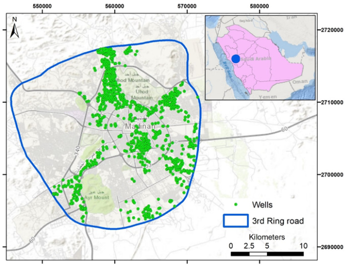 | Figure 1. Selected study area and well locations |
1053 wells are collected from urban populated areas in Madinah (inside the 3rd ring road). The data are collected from groundwater well locations and taken by two methods. For the private farms, the data are taken by the field visit and the location of the wells are determined by GPS with some quantitative information (i.e. well depth, water level, well diameter), this part of the data consists of about 83% of the total collected data. The rest of the data are extracted from houses with high cultivated areas using recent satellite images of the areas. Figure 1 shows the selected study area and the location of the groundwater wells.
3. Methodology
3.1. Assessing Clustering Tendency
Clustering methods divide the data into clusters even the data do not have any clusters. So, clustering tendency assessment is the first step in the cluster analysis, which should be used to evaluate the clustering analysis process validity. Assessing clustering tendency (ATC) measures the feasibility of the cluster analysis and whether a given data is clusterable. Two methods are used in this study; Hopkin's statistics and graphical method, which is visual assessment of cluster tendency (VAT). Hopkins statistics measures the spatial randomness of the dataset and can be computed as follows [9]:  | (1) |
where  is the distance between simulated point and its nearest neighbor,
  is the distance between data point and its nearest neighbor, and n is sample size. If the value of H is 0.5, this means that the data is uniformly distributed, while if H is less than 0.5 and close to zero, then the data is not uniformly distributed (i.e. contains meaningful clusters) [10, 11]. Small code in R programing language [12] is developed to compute Hopkin's statistics using “clustertend” R package [13].VAT plot can be constructed by first computing the Euclidean distance among the sample data and then reordering the distances where the similar objects are close to each other, then the VAT plot is developed. The presence of squared shaped dark blocks along the diagonal in a VAT image is an indication that the data set has cluster structures [14]. Small code in R programming language is written to develop the VAT plot using “factroextrac” R package [15].
3.2. Parameter Estimation
Estimating the input parameter for density-based clustering algorithms is still problematic and not yet solved. Density-based clustering algorithms usually require one or more input parameter, which are the minimum number of features (neighbors) per cluster (MinPts) and the search radius distance “ε” [16]. DBSCAN estimates the density by counting the number of points in a fixed-radius neighborhood and considers two points as connected, if they lie within each other’s neighborhood. A point is called “core point” if the neighborhood of radius (ε) contains at least MinPts points [17]. The required input parameter for the three selected algorithms is MinPts, which is the minimum number of features (neighbors) for each cluster. Too small MinPts selection produces high number of clusters and vice versa. The suggested value of MinPts in the literature is around 10 [8]. The value of the search radius distance (ε) input parameter is computed by constructing K-NN distance plot where the value of k is specified by the user and corresponds to MinPts and the best value of the search radius distance (ε) is around the sharp change occurs along the k-distance curve "the knee" [18]. The K-nn distance plot is constructed by developing code in R language using “dbscan” R package [19]. This package is also used to compute the three selected cluster algorithms. After estimating the two input paramters (MinPts and ε), the three density-based clustering algorithms are used to predict the clusters of groundwater well locations. Finally, the Convex Hulls polygons are plotted for each cluster to delineate the boundary of each groundwater aquifer.
4. Analysis and Results
4.1. Assessing Clustering Tendency
The computed Hopkin's statistics by using "clustertend" R package was found to be 0.12, which is close to zero and far below the threshold 0.5. This means that the well locations dataset is highly clusterable. VAT plot for the well location dataset is developed by using "factroextrac" R package and shown in Figure 2. The squared shaped dark blocks along the diagonal in a VAT image can be seen clearly, which is an indication that the well location data set has cluster structure.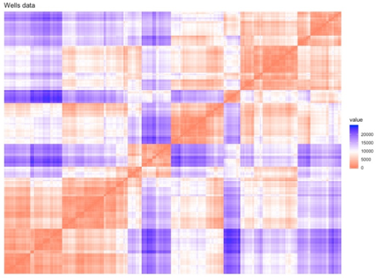 | Figure 2. Visual assessment of cluster tendency (VAT) of wells locations |
4.2. DBSCAN Clustering
The MinPts parameter is estimated as 10 features per clusters and the K-NN distance plot is developed using “dbscan” R package. Figure 3 shows that the search radius distance (ε) is about 1,000 m.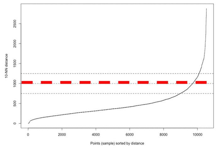 | Figure 3. K-NN Distance plot (using MinPts = 10) |
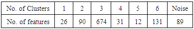
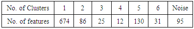
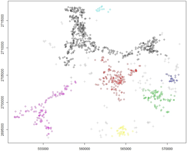
These two parameters are used to compute the DBSCAN, which produced 6 clusters with 89 locations as noises. Figure 4 shows the spatial clusters locations while Table 1 presents the number of features for each cluster. 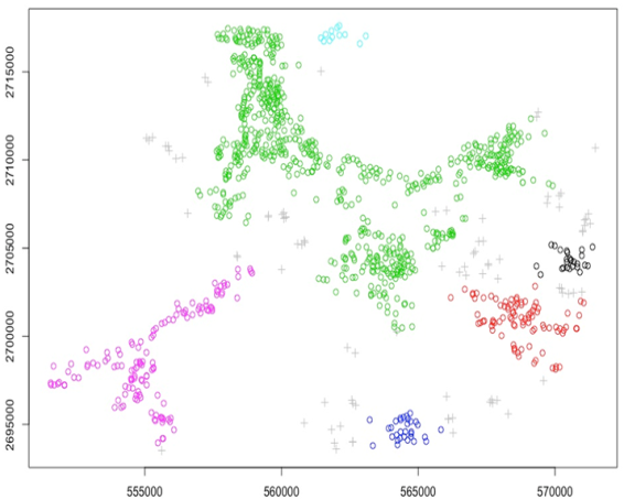 | Figure 4. Groundwater wells clustering using DBSCAN algorithm |
Table 1. Distribution of clusters per features using DBSCAN algorithm
 |
| |
|
4.3. HDBSCAN Clustering
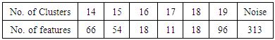
This algorithm needs only one parameter, which is MinPts, and it is set to 10, and hence, HDBSCAN algorithm produced 19 clusters with 313 locations that are considered as noises, which are relatively high. Table 2 presents the number of features for each cluster, while Figure 5 shows the location of these clusters.Table 2. Distribution of clusters per features using HDBSCAN algorithm
 |
| |
|
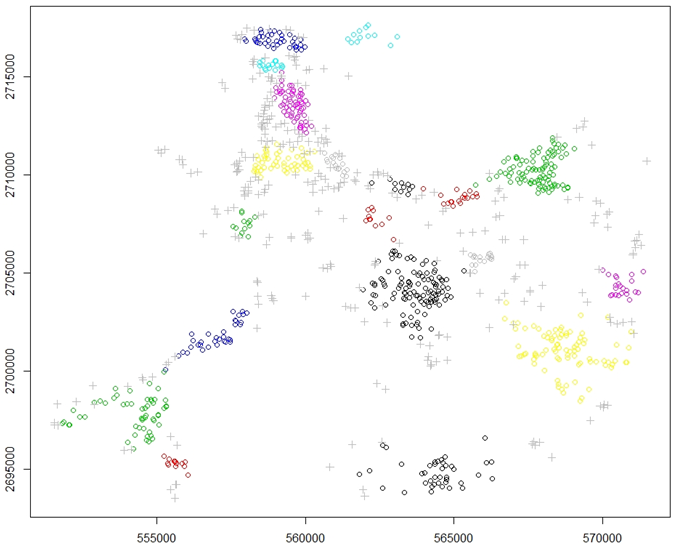 | Figure 5. Groundwater wells clustering using HDBSCAN algorithm |
4.4. OPTICS Clustering
This algorithm needs two input parameters, namely, MinPts that has different effects than DBSCAN algorithm [19], and Threshold to identify clusters (eps_cl <= eps). OPTICS algorithm produced 7 clusters with 95 locations as noises. Table 3 presents the number of features for each cluster, while Figure 6 shows these clusters location.Table 3. Distribution of clusters per features using OPTICS algorithm
 |
| |
|
 | Figure 6. Groundwater wells clustering using OPTICS algorithm |
4.5. Convex Hull Polygons
Each cluster in the three algorithms is delineated using convex Hull polygons, where each polygon is considered to represent one groundwater aquifer. Figure 7 shows the clusters delineation using convex Hull polygons for the three cluster algorithms.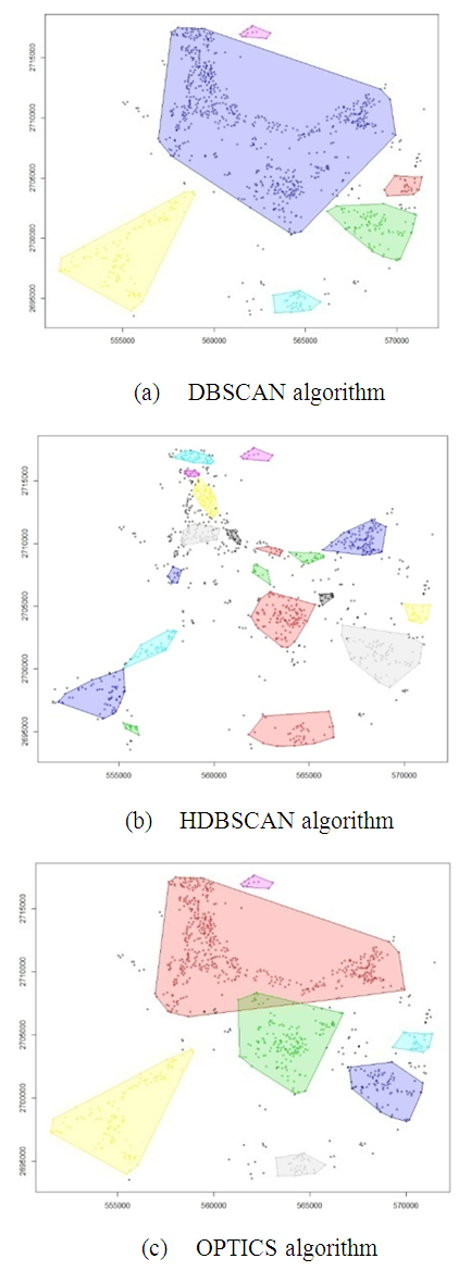 | Figure 7. Cluster delineation using convex hull polygons for the three cluster algorithms, (a) DBSCAN, (b) HDBSCAN, (c) OPTICS |
5. Conclusions
Groundwater well locations are considered as indicator for aquifer delineation using three spatial clustering approaches, which are DBSCAN, HDBSCAN and OPTICS. The application of these methodologies is based on more than one thousand wells in Madinah, Western KSA. Hopkin's statistics and VAT plot showed that the data has high clusterability (spatial randomness). The DBCAN and OPTICS algorithms produced very reasonable results with 6 and 7 clusters, respectively. It was found that the aquifers are located in the western south, south, eastern south, middle and north of the selected area. The results are expected to be beneficial for water resources planner and decision makers in cases of groundwater related projects.
References
| [1] | Parimala, M., Lopez, D., and Senthilkumar, N. C. (2011). A survey on density-based clustering algorithms for mining large spatial databases. International Journal of Advanced Science and Technology, 31(1), 59-66. |
| [2] | Popat, S. K., and Emmanuel, M. (2014). Review and comparative study of clustering techniques. International journal of computer science and information technologies, 5(1), 805-812. |
| [3] | Wierzchoń, S. and Kłopotek, M., (2018). Modern algorithms of cluster analysis, Studies in Big Data, Volume 34, Springer Nature Switzerland AG, pp 433. |
| [4] | Ester, M., Kriegel, H. P., Sander, J., and Xu, X. (1996). A density-based algorithm for discovering clusters in large spatial databases with noise. In Kdd (Vol. 96, No. 34, pp. 226-231). |
| [5] | Suthar, N., Rajput, I., and Gupta, V. (2013). A Technical survey on DBSCAN clustering algorithm. International Journal of Scientific and Engineering Research, 4(5). |
| [6] | Campello, R. J., Moulavi, D., and Sander, J. (2013). Density-based clustering based on hierarchical density estimates. In Pacific-Asia conference on knowledge discovery and data mining (pp. 160-172). Springer, Berlin, Heidelberg. |
| [7] | Ankerst, M. Breunig, M. M., Kriegel, H. P. and Sander, J. (1999). OPTICS: Ordering points to identify the clustering structure, in Proceedings of ACM-SIGMOD International Conference on Management of Data, Philadelphia, PA, 1999. (ACM Press, 1999), pp. 49–60. |
| [8] | Dubey, P., and Rajavat, A., (2016). Comparative study between density based clustering - dbscan and optics, Proceedings of 64th IRF International Conference, 16th October, 2016, Pune, India, ISBN: 978-93-86291-14-1. |
| [9] | Hopkins, B. and Skellam J. (1954). A new method for determining the type of distribution of plant individuals. Annals of Botany 18(2), pp213–227. |
| [10] | Banerjee, A., and Dave, R. N. (2004). Validating clusters using the Hopkins statistic. In Fuzzy systems, 2004. Proceedings. 2004 IEEE international conference on (Vol. 1, pp. 149-153). IEEE. |
| [11] | Adolfsson, A. Ackerman, M. and Brownstein, N. C. (2016). To cluster, or not to cluster: how to answer the question. In Proceedings of Knowledge Discovery from Data, Halifax, Nova Scotia, Canada, August 13–17 (TKDD‘17), 9 pages. |
| [12] | R Core Team (2013). R: A language and environment for statistical computing. R Foundation for Statistical Computing, Vienna, Austria. URL http://www.R-project.org/. |
| [13] | YiLan, L. and RuTong, Z. (2015). Clustertend: check the clustering tendency. R package version 1.4. |
| [14] | Bezdek, J. C., and Hathaway, R. J. (2002). VAT: A tool for visual assessment of (cluster) tendency. In Neural Networks, 2002. IJCNN'02. Proceedings of the 2002 International Joint Conference on (Vol. 3, pp. 2225-2230). IEEE. |
| [15] | Kassambara, A. and Mundt, F. (2017). Factoextra: extract and visualize the results of multivariate data analyses. R package version 1.0.5. |
| [16] | Chauhan, R., Batra, P., and Chaudhary, S. (2014). A survey of density based clustering algorithms, International journal of computer science and technology, Vol. 5, issues 2, 169-171. |
| [17] | Ester, M. (2014). Chapter 5: density-based clustering, In Charu, Aggrrwal, and Reddy (eds.) Data clustering: algorithms and applications, CRC Press. pp. 648. |
| [18] | Kassambara, A. (2017). Practical guide to cluster analysis in R: unsupervised machine learning (Vol. 1). STHDA. |
| [19] | Hahsler, M. and Piekenbrock, M. (2018). Dbscan: density based clustering of applications with Noise (DBSCAN) and related algorithms. R package version 1.1-2. https://CRAN.R-project.org/package=dbscan. |

 Abstract
 Reference
 Full-Text PDF
 Full-text HTML