1. Introduction

Ionosphere, part of the upper atmosphere of Earth extending from 60 km to 1500 km above the Earth’s surface, is a highly changing environment, both spatially and temporally. The variability of this environment depends mainly on Earth's rotation, season, solar and geomagnetic activity [1]. Many researches show that the ionospheric attitude during geomagnetic storms is varied from its normal attitude [2]. The geomagnetic storm makes thermospheric winds, inspires electric currents and changes the structure in the upper atmosphere. Each of them can produce a non-regular variation in the photoionization, recombination, and transport processes causing an irregular change in the electron concentration of the ionosphere. Some main effects are the significant change in the neutral wind circulation and atmospheric composition affecting the rate of production and loss of ionization, which caused the serve changes in TEC [3].

The significance of oversight the ionosphere layer lies in contributing useful understanding to the physics behind different space weather phenomena [4, 5, 6], in providing valuable insights into the possible causes of natural and man-made hazardous events such as earthquakes [7, 8, 9, 10]. Since its premier operation in 1978, GPS has certain to be an influential sensor for monitoring the ionosphere with wide spatial coverage and high temporal resolution [11, 12, 13, 14, 15]. The vertical Total Electron Content (vTEC) is usually the most widely used in presenting values of global ionosphere content density [16, 17]. IGS orderly produce the snapshots of the global vTEC in the form of Global Ionosphere Maps (GIMs) [14, 18]. GIMs can extended ionospheric TEC with 5° and 2.5° spatial resolution in longitude and latitude, respectively, and a temporal resolution of few minutes to several hours in real-time, rapid and final modes. Although the real-time GIM produces have been offered by the IGS, users now can only outlet the rapid and final GIMs with a latency of few days [19]. GIM in IONEX format can be downloaded from IGS analysis center site ‘ftp://cddis.gsfc.nasa.gov/gps/products/ionex/’ in TECU units where 1 TECU = 1016 el/m². There are four IGS IAACs have been frequently participating GIM products to the IGS ionosphere working group since 1998, these centers including CODE, Universitat Politècnica de Catalunya/IonSAT (UPC), Jet Propulsion Laboratory (JPL), European Space Operations Center of European Space Agency (ESA) [13, 18, 20, 21].

This study aims to have an accurate TEC mapping tool that can use local stations dual frequency GPS observations to produce TEC values with a temporal resolution of 1 h. This tool was written under MATLAB environment and can be used globally to produce GIMs from local GPS networks in several areas with low number of IGS stations or without. Firstly, values of TEC from this tool were validated using IGS stations and CODE’s GIMs. Seven regional stations GPS observations distributed over Egypt were used to estimate TEC values over Egypt.

2. Ionospheric Model

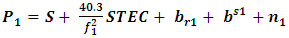
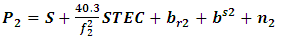
As ionosphere delay is frequency dependent, it can be obtained using dual frequency observations. The pseudorange measurements observation equations for dual frequency GPS can be expressed as [20]:

(1)

(2)

Where P₁ and P₂ are pseudorange measurements in L₁ and L₂ bands, S is the term not related to frequency, i.e. distance, tropospheric delay and clock errors, f₁ and f₂ are carrier frequencies in L₁ and L₂ bands, b_s and b_r are satellite and receiver biases respectively, Slant Total Electron Content (STEC) is TEC along the signal pass, and n₁ and n₂ are measurement noises.

For ionosphere study, the geometry-free linear combination between pseudorange and carrier phase is normally formed to remove range related term. Both dual-frequency pseudorange code observations (Melbourne–Wubeena combination) and ionospheric residual observations are used to detect cycle slips and gross errors [22]:

(3)

Where: Δb_s and Δb_r are the Differential Code Biases “DCB” for satellite and receiver.

In the two-dimensional modeling process, it is usually assumed that the free electrons of the entire ionosphere are concentrated in the thin layer at the height with the maximum electron density. Based on the hypothesis of the single-layer shell model, the STEC value along the path can be transformed into the vTEC at the Ionospheric Pierce Point (IPP) by using the ionospheric mapping function [23]:

(4)

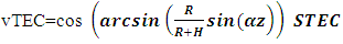
Where R is the radius of the Earth = 6371 km, is the attitude of the ionosphere thin shell (assumed as used by CODE=506.7 km, 0.9782 [24]), is elevation angle at the ground station.

The ionospheric model based on the Spherical Harmonic can be expressed as [24]:

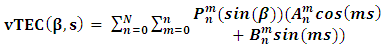(5)

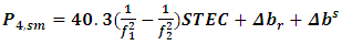
Where: β is the geocentric latitude of IPPs (Ionosphere Peirce Point), s is the solar fixed longitude of IPPs, N is the degree of the spherical function, m is the order of spherical harmonic function, is regularization Legendre series and and are the estimated spherical harmonics coefficients. The height of the ionospheric single layer model in the current study is set to equal 506.7 km, as used by CODE, and 4-order and 4-degree Spherical Harmonic expansion are used to establish the model. The observations with the elevation angle below 10° are masked and removed. In case the GPS raw data do not include the P₁ observation (Non-cross correlation receiver type), the P₁-C₁ correction provided by IGS to modify the C₁ observation is used, and the observation combination between P₁ and P₂ can be obtained. As there is a huge number of observations, the spherical harmonic coefficient and the DCB of both P₁ and P₂ can be estimated according to the weighted least square method. The used weight function is based upon a function of elevation angle. Finally, the vTEC and DCB can be determined.

3. Data Used

As mentioned before, the main objective of the current study is to validate the GTM resulted from the developed model with related results produced by CODE’s GIMs. After the validity process, the developed modes was used to estimate TEC using regional GPS receivers network like Egypt network used here. To check the performance of the model in different Circumstances of TEC variation, TEC values of selected area from 0° to 20° longitude and from 42.5° to 55° latitude will be estimated in stormy and quiet days. Figure 1 shows the data that was used for validation process. This data is produced by 10 IGS stations namely, BRUX, FFMJ, GOPE, HUEG, LEIJ, OBE4, POTS, PTBB, WSRT and WTZZ.

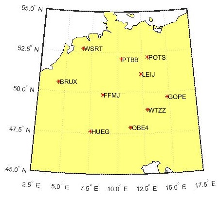Figure 1. Distribution of IGS stations

The selected stormy days are 7-10-2015, 8-5-2016 and 8-9-2018. Figure 2 (a, b and c) shows the values of Kp of the selected stormy days. The K-index, and by extension the Planetary K-index, are used to characterize the magnitude of geomagnetic storms. Kp is an excellent indicator of disturbances in the Earth's magnetic field and is used by SWPC (Space Weather Prediction Center) to decide whether geomagnetic alerts and warnings need to be issued for users who are affected by these disturbances [25].

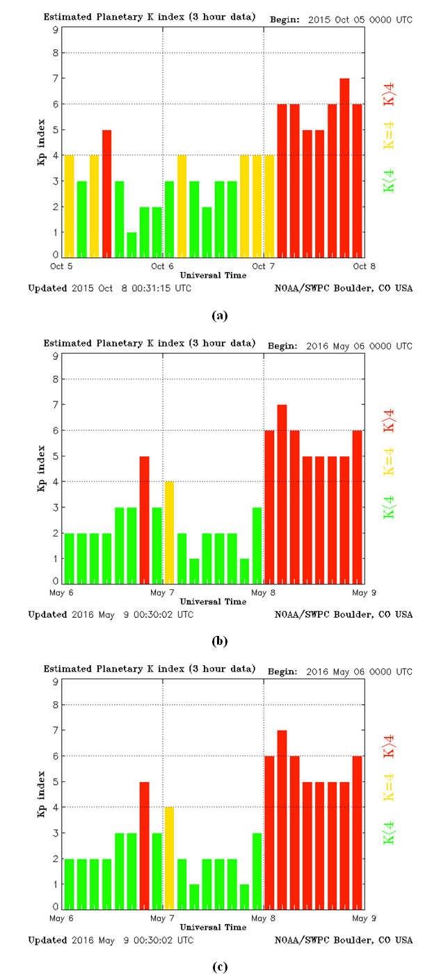Figure 2. The Kp values of the selected stormy days, (a) at 7-10-2015, (b) at 8-5-2016 and (c) at 8-9-2017 [26]

The Kp-index ranges from 0 to 9 where a value of 0 means that there is very little geomagnetic activity and a value of 9 means extreme geomagnetic storming. NOAA uses a five-level system called the G-scale shown in figure 2 [25].

NOAA uses a five-level system called the G-scale, to indicate the severity of geomagnetic activity. This scale ranges from G1 to G5, with G1 being the lowest level and G5 being the highest level. G0 indicates below storm for Kp=4 and lower, G1 indicates minor storm when Kp=5, G2 indicates moderate storm for Kp=6, G3 indicates strong storm for Kp=7, G4 indicates serve storm for serve storm for Kp=8 and G5 indicates extreme storm when Kp=9 (Space Weather, 2019). For selected days, storm levels on 07 Oct 2015, active to G2 (Moderate) geomagnetic storm, on 08 May 2016 G1-G3 (Minor-Strong) geomagnetic storms were observed and finally, The geomagnetic field responded with active to G4 (severe) storm levels on 08 Sep [25].

On the other hand, the selected quiet days are 10-9-2017, 6-9-2018 and 8-9-2018. NOAA indicated all of those three days as the geomagnetic field is quiet. For each day of data, the following files were downloaded, the Receiver Independent Exchange (RINEX) format according to the selected stations (figure 1) downloaded from (ftp://garner.ucsd.edu/rinex) and precise ephemerides (SP3) files of test days and P₁-C₁ correction downloaded from (http://www.GPScalendar.com/index.html). In addition, IONosphere Map EXchange Format (IONEX) files of CODE are downloaded from (ftp://cddis.gsfc.nasa.gov/GPS/products/ionex/).

Figure (3) depicts seven selected locations of GPS station of a regional network in Egypt at day 7-6-2015 to estimate TEC values over Egypt. The network Consisting of seven ground receivers named as ABSM, ALAM, ARSH, ASWN, BORG, MTRH and SAID distributed according figure 3. SP3, P1-C1 correction and IONEX files of this day also downloaded from the past mentioned websites.

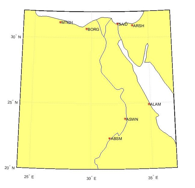Figure 3. Distribution of regional GPS stations of Egypt

4. Validation Results

The model is applied to the mentioned above groups of days. Table 1 and table 2 give the values of mean TEC values of CODE and mean values of the output TEC of GTM model every 1 h in TECU (TEC Unit= 10¹⁶ electron/m³, 1 TECU= 0.163 m and 0.267 m in L₁ and L₂ frequencies respectively (Ovstedal, 2002)) for the selected area for stormy and quiet days. Also, the table gives the Mean and Standard Deviation of the Mean (SDM) of the TEC results for each hour that used often to reveal the amount of variation or dispersion of a set of data values. Mean and SDM equations are described by the following functions.

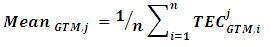(6)

(7)

Where j is the time by hours from 1 to 24 and n is the number of TEC results.

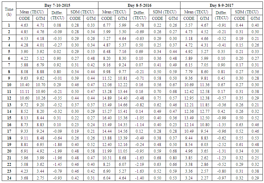Table 1. Statistical values of CODE and GTM TEC results for the selected stormy days

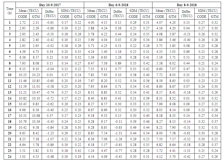Table 2. Statistical values of CODE and GTM TEC results for the selected quiet days

As it is demonstrated in the above two tables, it can be seen that TEC values start with small values at the beginning of the day and increase gradually till the mid of the day and decrease gradually till the end of the day. The gradual increase in TEC to a maximum value at peak hours of the day has been attributed to the presence of magnetic flux after sunrise which leading to increase in ionization due to increasing thermospheric temperatures. TEC values of stormy days, of course, are larger than that of the quiet geomagnetic days that agreed with that mentioned in section 1.

Table 3. Statistical values of CODE and GTM TEC results for day 7-6-2015

Also, the difference (differ.) between minimum and maximum values of TEC at stormy days is greater than of those of quiet days. The maximum difference value between CODE and GTM model seen in stormy days is 2.52 TECU otherwise almost difference values are less than 1 TECU.

On the other side, the values of SDM that define the dispersion of the results of CODE and GTM are almost close to each other. The maximum between CODE and GTM can be detected is 0.24 TECU otherwise almost values of the three stormy days are less than 0.1 TECU. For the three quiet days the maximum difference between CODE and GTM TEC results is 1.31 TECU otherwise almost differences are less than 1 TECU. Maximum difference of SDM of CODE and GTM is 0.24 TECU and almost differences are less than 0.1 TECU. These results of stormy and quiet days show how TEC values of CODE and those estimated from GTM model are close to each other.

5. Egypt TEC Mapping

After the make sure of the Convergence of results of GTM with those of CODE-one of IAAC-it is time to estimate TEC values over Egypt from its regional 24h working receivers. Firstly, TEC values are estimated using GTM and then ARCMap 10.6 was used to draw TEC maps. Borders of the maps are from 24° to 37° longitude and from 20° to 32° latitude with 1h temporal resolution of day 7-6-2015. The following figure 4 shows these TEC maps.

The shown 24 TEC maps (figure 4) give a snap shot of the ionosphere distribution over Egypt country borders every 1 hour. Maps show near equally distribution of TEC over Egypt in all time of that day except the afternoon hours from 12h to 16h. That can be observed from the divergence of contour lines of in steady hours and convergence of them in afternoon hours. The highest values of contour TEC values are calculated from real GPS observation not interpolated points.

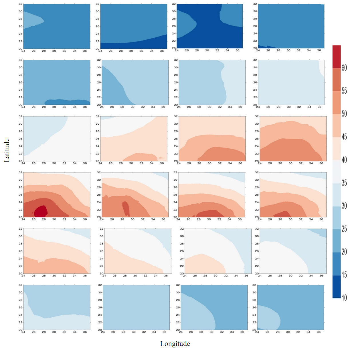Figure 4. TEC maps over Egypt country start from 1h to 24h of day 7-6-2015

6. Conclusions

In this study, a global TEC mapping model was developed to monitor ionosphere changing with 1 h temporal resolution based on dual frequency GPS receivers. The spherical harmonic expansion technique was used as the mathematical model for the global ionosphere model with degree and order of 4. Statistical values of our model are very close to those of CODE-one of the international ionosphere ACs that usually provide the TEC map. This model shows good results in both stormy and quiet days. Using 1 h maps interval is more useful for quickly recognize the ionosphere variation, especially in stormy days. The GTM model can be used regionally to estimate the ionospheric delay of the pseudo range.