1. Introduction

Current literature shows the need to revise our understanding of external migration to appraise future conditions of sustainability in socioecological production landscapes (SEPLs) of mountainous regions (Abrams et al. 2012; Fitzhugh et al. 2018). Assessment of emigration impact is particularly relevant where conflicting views of biocultural conservation are present. On the one hand, the imperative of job availability to provide for the essential needs of the family and the lack of paying jobs in the area. On the other hand, the increasing consumerism in the site of origin pushes for the need to provide cash to energize transactions and introduce locals into the modernity of Latin American landscapes (Sánchez et al. 2017). Scholars debated over the significance of rural-to-urban migration to the future of Andean towns (Grau & Aide 2007), and broaden our inquiry to grapple with the outflow of people from the less developed countries toward the Global North (Zlotnik 1995; Schiff 1999; Wihtol de Wenden 2018).

This migratory trend from the rural areas to the nearby cities has been in place since colonial times when small towns benefitted from the newly created republics and consolidated the governmentality of mountain areas following European or North American schemes of development, making the phenomenon of primacy noteworthy throughout the hemisphere (Bloch & Dona 2018). Recent migratory dynamics of southern Ecuador have highlighted the effect of migration and mobility as determinants of the new rurality (Rivera-Muñoz & Meulder 2018). Moreover, the vulnerability of rural territories to global change determine alternative scenarios that collide with the paradox of depopulated peasantries and the affluent expat newcomers (Rebaï & Alvarado 2018). We frame our research within the inverse amenity migration paradigm (Moss 2006) that investigates the trope of emigration forcing changes associated with high amenity areas in mountain environments, exacerbating the clash of global economic trends in the Anthropocene promoting of local extirpation instead of the inclusion of foreign arrivals into the community (Mata-Codesal 2018). Facing the predicament of lacking jobs or menial salaries, the dilemma of development and conservation, typical of Neotropical mountainscapes, becomes central to inform on sustainable development scenarios amidst mobility trends and heritage preservation (Sarmiento & Frolich 2012).

In the socio-ecological dynamics of globalized economies, the movement of people and goods has prompted a realignment of destination choice. We hypothesize that the rich migrants of the global north are going to destinations that suffer with joblessness and lack of education, making poor locals to engage in emigration waves from the global south towards active labor-seeking northern markets. The foreign amenity immigrants readily discover the geospatial memory of bucolic images imprinted in the poor emigrants, generating oxymora of the haves and the have-nots distributed in the receptive, often stressed, mountain landscapes. Therefore, we need to assess whether lack of jobs and poor educational level are factors that press emigration trends that could, in turn, bring buoyancy to those left behind because of remittance input as time passes.

Not only do social, economic and demographic processes morph over the years but they also vary spatially. In other words, they are not static as they depend on when and where the measure is taken. The use of census data facilitates comparison between data points separated by roughly ten-year intervals. Through statistical analyses we know the degree of relationship between different variables, but the variability of these associations in a map is not known. To understand these changes, it is necessary to use spatial-statistical data and the techniques of weighted geographical regression (GWR) to visualize data relationships. In addition, to better visualize the results of these spatial regressions, a second method is added: spatial interpolation methods (SIM). Both techniques allow for a more precise and unbiased geospatial assessment of the target phenomenon. The rural landscape of Cañar province is a patchwork mosaic of remnant Andean forests, agricultural fields, grassland or pastureland and small towns and villages in the interAndean valleys, considered as SEPLs. The larger concentration of urban area is located around the city of Azogues with conurbated towns of Déleg, Cañar, El Tambo and Biblián. Because of the recent phenomenon of remittance-based affluence and the target destination of amenity receiving migrants from the global north to these areas of Ecuador, we decided to analyze the drivers of migration affecting the city of Biblián as a case study (Figure 1).

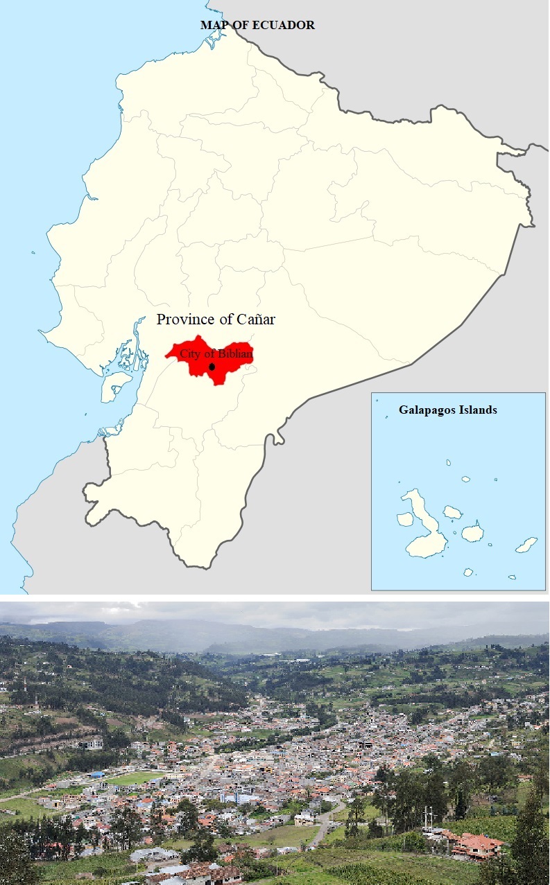Figure 1. Study Area: location and picture of the city of Biblián

2. International Migration Framework in Biblián

International migration has increased in recent decades particularly from low income nations towards high-income countries (Ratha, Shaw & William 2007). Thus, migration is a very important indicator of a country’s socio-economic well being and development. Migration flows are movements of people and especially of labor from countries with socio-economic problems to countries where employment and wages are better. There are five explanations for the causality of international migration processes that are happening in the South Central Andes of Ecuador, also called the Austro region (Arango 2017), namely: neoclassic economic theory, labor market theory, new economics of labor migration, relative deprivation theory and world systems theory.

1) Migration explained by the Neoclassic Economic Theory: This theory states that the reason for labor-related international migration are wage differences among countries (Borjas 1989). The income differences are linked to differences in labor demand and supply. Areas with a lot of capital but a shortage of labor are characterized by high relative wages while areas with a lack of enough capital and with an abundance of workers are characterized by low wages. Therefore, fluxes of labor tend to move from low-income to high-wage areas. These migration processes generate changes in the nations that lose workers as well as in the receiving nations. Migration determines that workers are now less scarce at the destination but more scarce at their countries of origin and capital begins to move from rich into poor nations via remittances thereby generating a process of “factor price equalization” (O’Rourke & Sinnott 2006). At the micro-level, neo-classical migration models state that migrants are rational individuals who are willing to move after they calculate their costs and benefits These individuals have free choice and full access to information, therefore, they move to areas where they can be the most productive when measured by incomes. Obviously, this capacity depends on the specific knowledge and skills that different migrants have and of specific structures of the various labor markets.

2) Migration due to the dual labor market theory: This theory states that international migration is caused by pull factors in the richest nations (Piore 1970), assuming that the labor markets in these rich countries are segmented in two parts (Reich, Gordon & Edwards 1973): a) a labor market characterized for being based on high-skilled labor and b) another labor-intensive sector but requiring non-qualified workers. The secondary labor market is the one that generates international migration from less developed countries into more developed nations because native individuals do not want to work in low paying jobs, generating a pull of immigrant workers to industrialized countries that fill the lowest rung of the labor market.

3) Migration explained by the new economics of labor migration: This theory states that international migration flows need to be explained not just at the individual level but, instead, to take into account wider social entities such as the household or kinship (Stark & Bloom 1985). Therefore, migration is the result of a household taking a risk due to its insufficient income. The household in search of additional money sends one or more of its members abroad to receive in exchange remittances that are sent back by their absent relatives. These monetary fluxes have broader effects on the economy of the sending and receiving countries (Taylor 1999). Before moving, migrant workers learn about the economic situation of the target countries before moving there, establish contracts or liaisons with intermediaries that facilitate the move (c.f., coyotes) as well as migration support networks in the new nations help them to settle in target labor intensive markets.

4) Migration because of the relative deprivation theory: This theory states that, because people are aware of the income difference between neighboring households in their migrant-sending towns or rural areas (Walker & Pettigrew 1984), this fact generates a strong desire to emigrate to the richer country. Due to past emigrations, income inequalities in sending communities become increasingly greater and the incentive for departure increases among their population (Stark & Taylor 1991). Successful emigrants may serve as an example for their neighbors and their families so that future migrants hope to achieve the same level of success. Also, successful migrants use their remittances to buy or build up better houses for their families as well as to invest in existing businesses or to create new ones.

5) Migration explained by the world systems theory: This theory states that interactions among different countries or societies are the main factor in social changes within communities (Arango 2000). For example, trade between two countries can causes economic decline in one of them, creating an incentive to migrate to the country with a better economy such as former colonies with their motherlands. Even after decolonization, economic dependence from former colonies on more powerful countries still remains a motivating factor for preferential (c.f., quotas) procedence. The rich countries import goods characterized for being labor-intensive, generating an increase in employment of unskilled workers in the poor nations and thus decreasing the migration of workers, while the developed nations export capital-intensive goods to undeveloped countries generating the need for circulating capital to buy them (Schiller, Basch & Blanc-Szanton 1992).

All five migration theories adapt well to explain the causality of the international migration process in the city of Biblián and in other poor areas (urban and rural) of the Austro region. From an economic perspective, international migration is directly related to differences in job opportunities, per-capita income and living standards across countries; especially between the wealthy north and the poor south (Solimano, 2010). Ecuador has a per-capita Gross Domestic Product income that is several times lower than other countries (e.g., in 2015, per-capita income in Ecuador was barely US $ 6,100. annually compared to US $ 25,820 in Spain or US $ 56,720 in the United States, both are the countries with more migrants of Ecuadorian nationality) (International Monetary Fund 2018).

3. Research Objectives

Recently, papers have increasingly been written using a variety of new geomatic tools. Therefore, GIS, remote sensing, photogrammetry, digital cartography and modelling have created new achievements as well as new challengers for researchers and planners worldwide. Specifically, the spatial technique GWR helps to determine relations between variables from the natural and human sciences that before were hidden to the human eye; in the same token, spatial interpolations show intricate patterns of different kinds of phenomena, and the use of both tools combined is the clue to understand the world spatially, becoming a true revolution in the scientific understanding of the fundamental processes that constantly shape our societies, as well as the natural world. These two spatial analysis methods have been applied mostly independently to a multitude of disciplines, such as geology, edaphology, biology, ecology, archeology, economics, demographics, epidemiology, etc. as well as in interdisciplinary research, with very positive scientific results, but when GWR and SIM are integrated, they constitute one of the most powerful approaches to understand reality, the main mission of science.

In order to explore our hypothesized oxymoron of geospatial memory, we seek to determine which areas of the city of Biblián have people with different levels of education (from no instruction, K-12, or to the fourth level: masters or doctorates), income sourcing (paid or unpaid work), as well as to determine which areas of Biblián have people who have emigrated abroad. With the geovisualization outputs through choropleth maps according to the information obtained in the MIMM Census and GIS of Biblián, we want to determine, through weighted spatial regressions (GWR), the degree of association between the independent variables: levels of education and paid or unpaid work, in relation to the dependent variable: emigration abroad. Finally, to better understand the behavior of these variables and these relationships, spatial interpolations were made that changed the choropleth maps at the building level (including horizontal property) by isopleth maps of continuous surfaces, through which the visualization of all these phenomena improves, allowing robust analysis.

4. Methods

4.1. Study Area

We have selected as our study area the inter-Andean valley where the city of Biblián is located in the province of Cañar, in the southern highlands of Ecuador (Fig. 1). We had three reasons to choose Biblián to carry out the census of the Migration Impact Monitoring Mechanism (MIMM) in the month of March 2015 Firstly, the population of the city of Biblián according to the 2010 National Population and Housing Census showed 5,496 people (INEC, 2010); since it was not too big, it had the resources to carry out a new census five years later in all its urban area. Secondly according to data from the consecutive National Population and Housing Censuses of the years 2001 and 2010, it was found that Biblián’s province was, on both occasions, among the 20 nationwide with the highest incidence of international emigration (Herrera, Moncayo & Escobar 2012); and, thirdly, the close proximity between Biblián and the city of Cuenca, (only 38 Km) and the paved highway, which facilitated logistics of the MIMM census, since surveyors and researchers belonged to the University of Cuenca.

5. Data Analysis

We used ArcMap software, part of the ArcGIS package from ESRI, and its extensions or tools for Space Analysis and Spatial Statistics, which consists of three phases:

1) the creation of the Geographical Information System (GIS) based on the update of the urban cadaster of Biblián and linked to the building level (some of which include horizontal property-departments or rooms) with the statistical database of the census of the Mechanism of Migration Impact Monitoring (MIMM) and selection of two independent variables-education levels (question Q22 of the MIMM survey) and paid work (question Q50 of the same survey) with respect to its incidence in a dependent variable: international emigration (Q74) ad with generation of choropleth maps where these three variables are represented cartographically;

2) generation of continuous surfaces through spatial interpolation to better visualize the interactive behavior of these three variables and;

3) spatial regression in an individual and joint way between data of the independent variables (Q22 and Q50) in relation to the dependent variable (Q74) which finally appear again through spatial interpolations in continuous surfaces whose relational influence or association is easy to visualize and understand.

5.1. Creation of the Statistical-Geographical Database and Selection of Variables

As a preliminary procedure to the census of the Migration Impact Monitoring Mechanism (MIMM) of 2015 carried out in Biblián, the errors of the cadastral map made in this city in 2010 were corrected; then, this revised cadastral file was converted from AutoCAD DXF (Drawing Exchange Format) to Shapefile format to be later worked in ArcGIS software(Li-jia, 2007) and thus create the corresponding Geographic Information System (GIS) projected through the World Geodetic System of 1984 (WGS84), proyección Universal Transversal de Mercator (UTM) and Zona 17th Sur (Seeber, 2003).

The MIMM census was based on the collection of statistical surveys consisting of 278 questions (Verdezoto, Abainza, Calfat & Neira 2015) made to each of the 1,295 households in the city of Biblián in 1,185 buildings existing within the urban perimeter which consequently generated a large statistical-spatial database with specific information at the level of homes and buildings which would include horizontal property because they are spatially located within them. This included demographic information, among them, education, work, migratory history of international and internal migration, returnees, enterprises, family structure, communication, economic and social remittances, income and expenses, characteristics and conditions of housing and personal property. The main objective of MIMM was to generate relevant information to be used through statistical and spatial analysis and thus understand the associations and consequences of migratory flows on society, and finally to make recommendations aimed at solving problems through public policies that may be applied in a real context thus contributing to local development and conservation.

This statistical database was introduced within the GIS (Longley 2005), where all household variables were linked to each of the 1,185 existing buildings (included within the same 135 horizontal properties) in Biblián (an average of 1.09 homes for each dwelling), the same ones that are represented by irregular polygons (according to the vector model) (Raper & Maguire 1992), that is to say that some buildings contained a single home, while others could contain several homes inside, especially because of horizontal property ownership. Therefore, statistically the elementary units are the homes, while spatially the basic unit is each building and each horizontal property inside, both located within a given registered property.

In accordance with the Third Principle of the Code of Good Statistical Practices of Ecuador (INEC 2000) and specifically in order to protect the confidentiality of the data corresponding to the persons who answered the questions and to keep the confidentiality of the MIMM census data safe, the original positions of the polygons that represent buildings were modified, moving them slightly, about twenty-five meters in random directions, changes that obviously affect all the maps created in this investigation.

Three weeks after the MMIM census was carried out, in order to validate the authenticity of the data, a small survey based on the same questions was carried out in the city of Biblián. This sample was carried out in 295 households with a confidence level of 95% and a 5% margin of error. The results for the three variables used in this study were the following: education levels (Q22) had an error of 2.17%, paid work (Q50) showed the highest error of 5.02% and the error for international emigration (Q74) was 4.16%. The reason for the highest error level in the variables of paid work and international emigration were due to the fact that many people were less than truthful because they feared that the results of this survey could be used by the local and national government to raise taxes or that the data would be sent to the United States embassy or to the United States Citizenship and Immigration Services (USCIS).

5.2. Spatial Regression

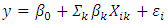
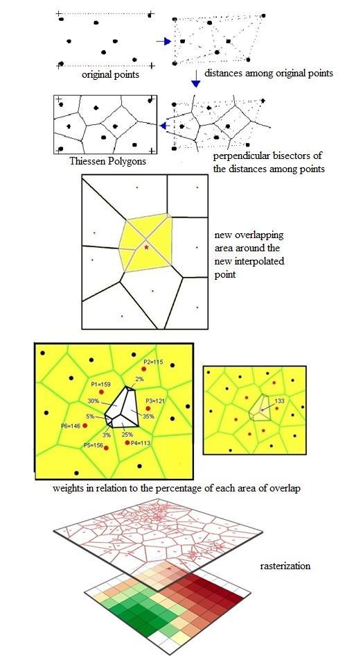
For a long time ago, there has been interest in local forms of analysis and spatial modeling (Anselin, 1995) since it is known that global models produce parameter estimates that represent a type of "average" behavior and, therefore, are very limited in understanding behaviors that vary in space. Statistics and local models provide us with the equivalent of a microscope; they are tools that allow the analysis in great detail of relationships and spatial patterns. Without them, the image presented by global statistics is characterized by uniformity and lack of variation in space.

Local statistical analysis of spatial data must deal with two potential types of local variation: the local relationship that is measured in the attributed space and the local relationship that is measured in the geographical space. In addition, the variations in the geographical space vary in two dimensions, instead of only in one.

By their nature, global statistics show similarities, while local statistics emphasize differences in space. On the other hand, global statistics usually have a mean value, a standard deviation and a measure of spatial autocorrelation in a data set (Cliff and Ord 1970) while local statistics have different values that are the result of existing relationships in the vicinity that occur in different locations within a study area.

Consequently, global statistics are not part of maps or are not conducive to being analyzed within a GIS, because they consist of unique values. Contrastingly, from local statistics, maps can be generated and examined more thoroughly within a GIS in which a pattern that reflects the different spatial variations of the causal relationship between two variables is manifested.

The Geographically Weighted Regression (GWR) is based on multiple and independent equations that incorporate both explanatory and dependent variables within a certain bandwidth from a Kernel (Wheeler 2014), from which specific decay patterns of distance are formed from their origin (Stewart Fotheringham et al. 2003a). These local studies also produce a table with different diagnostic values in a representation scheme with colors that vary between blue (high correlation) and red (low correlation) applied to the residuals of the model.

The dependent and explanatory variables contain a variety of values each and the analysis of spatial regression (GWR) begins by applying a simple regression model (Ordinary Least Squares or OLS) but local, resulting in values that are grouped or not spatially, and when this happens, a local association or relationship is generated.

The GWR is a technique used to explore spatial heterogeneity or variation in the study area (Stewart Fotheringham et al., 2003). To understand the causal relationships between variables (Brunsdon et al. 1998), this method is constructed by statistical-spatial indicators similar to those used in the linear regression:

(1)

But the GWR uses a global model, where it is assumed that the relationship between the independent and dependent variables is constant in each location (measurements in spatial coordinates ) in the whole study area, while the values of and are the same (McMillen 2004). The residuals of this model are instead independent and different from each other and are normally distributed through an arithmetic mean of zero (Charlton et al. 2009). The Weighted Geographical Regression (GWR) allows local values to be estimated instead of global parameters, and its formula is as follows:

(2)

Where correspond to the coordinates of each point in space, that is, a continuous surface of values that change in space and that represent the existing relationship between the independent variable and the dependent one is generated. In the GWR, each data point is weighted by its distance from the regression point; this means that the weight of the data has a maximum when it shares the same location as the regression point, but this weight decreases continuously as the distance increases. Therefore, data points closer to the regression point have more weight in the regression than the data points furthest away.

The results of the GWR are sensitive to the distance of the weighting function chosen and graphically the method consists in adjusting a Gaussian spatial kernel to the data (Babaud et al. 1986) and the result is a surface of different estimates (Fig. 2).

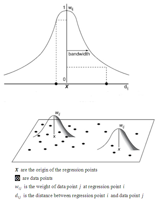Figure 2. GWR with fixed spatial kernels (Source: Stewart Fotheringham et al. 2003b)

There are other similar scientific articles that also have applied the GWR method in jobs, education and migration for example:

a) Li, Corcoran, Pullar, Robson, & Stimson (2009), were able to use GWR based on a combination of seven independent variables: 1) population; 2) location workforce; 3) location quotient; 4) proportion of land zoned for services or industries; 5) distance to the main shopping center or main activity center; 6) number of accommodations, café and restaurants and number of jobs in finance; 7) insurance, property, and business services to predict spatially disaggregate retail jobs at 289 statistical local areas (the equivalent of census tracts in the United States) in South East Queensland, Australia for years 2001, 2006, 2011, 2016, 2021 and 2026.

b) Lewandowska-Gwarda (2018) applied a GWR method in 380 districts in Poland. In this case, nine independent variables were used: 1) number of business entities entered in the register per 10,000 people; 2) districts’ budgetary incomes per capita in the Polish zloty (PLN); 3) emigration level or outflow of individuals abroad per 10,000 people; 4) feminization rate or number of women per 100 men; 5) capital investments in enterprises for each resident of economically productive age; 6) internal migration level or outflow of individuals per 10,000 people; 7) number of job offers per 10,000 people of economically productive age; 8) budgetary expenditures of municipalities and towns with district rights on social assistance per capita in PLN and 8) average wages in PLN to predict unemployment in Poland in 2015.

c) Nelson (2008) also used GWR in the continental United States at the county level using the following six independent variables from different data sources: 1) natural amenities; 2) married couples with no children, immigration rate, 3) domestic migration rate, 4) median home value, 5) metropolitan classifications and 6) social security exempt to predict life-course influences on non-earning income migration.

d) Partridge, Rickman, Ali, & Olfert (2008) applied a GWR method at the county level in the continental United States using thirty-eight independent variables: 1) average January temperature; 2) average January sunshine; 3) average July humidity; 4) typography; 5) percentage of water area; 6) agriculture share; 7) goods share; 8) percentage of immigrated over 1985–1990; 9) percentage of high school graduate; 10) percentage of people with some college education; 11) percentage of associate degrees; 12) percentage of college graduates; 13) percentage of African Americans; 14) percentage of Native Americans; 15) percentage of Anglo-Americans; 16) percentage of Asian pacific people; 17) percentage of Hispanics; 18) percentage of other ethnicities; 19) percentage of people under 6 years; 20) percentage of people from 7–17 years; 21) percentage of people 18–24 years; 22) percentage of people 55–59 years; 23) percentage of people 60–64 years; 24) percentage of people over 65 years; 25) percentage of unemployment; 26) median household income; 27) population density in 1990; 28) industry mix employment growth; 29) population living in surrounding counties in 1990; 30) percentage of unemployment in surrounding counties; 31) median household income in surrounding counties; 32) industry mixed employment growth in surrounding counties; 33) population of the nearest urban center in 1990; 34) distance to nearest urban center; 35) incidental distance to the nearest metropolitan area in kilometers; 36) incidental distance to the nearest metropolitan area with a population of at least 250,000 inhabitants in 1990; 37) incidental distance to the nearest metropolitan area with a population of at least 500,000 inhabitants in 1990; and 38) incidental distance to the nearest metropolitan area with a population of at least 1,500,000 inhabitants in 1990 to predict nonmetropolitan county employment growth dynamics from 1990 to 2004.

e) Wang (2007) used a spatial regression technique in Cleveland, Ohio at the census tract level where the following seven variables were selected as the independent ones: 1) black female heads of households; 2) unemployed residents without high school diploma; 3) mean family income; 4) families below the poverty level; 5) renter-occupied homes; 6) residents who moved in last 5 years; 7) households with one person per room, to predict accessibility to jobs in disadvantaged neighborhoods.

f) Ansong, Ansong, Ampomah, & Adjabeng (2015) used GWR to predict spatial inequality in academic achievement in Ghana based on the 2013 Basic Education Certificate Examination (BECE) results compiled by the Ghana Education Service. The eight independent variables used for this prediction were: 1) household size; 2) proportion of a population living in urban areas; 3) male employment; 4) female employment; 5) connectivity to electricity; 6) male literacy; 7) female literacy; 8) pedagogical resource index and 9) classroom congestion index.

g) Harris, Singleton, Grose, Brunsdon, & Longley (2010) used the following five independent variables: 1) population enrolled in higher education under 21 years; 2) people with no qualifications; 3) people under 18 still receiving child benefits, number of post 16 yr. qualifications; 4) average KS4 points; 5) four or more cars per household, and 6) percentage of Asian people in relation to the total population derived from the 2001 census and from the 2007 Index of Multiple Deprivation and using GWR. Using this they were able to model participation rates of higher education in England.

h) Fotheringham, Charlton, & Brunsdon (2001) based on a set of standardized tests administered to pupils from the ages of 7 to 11 years for 3,687 schools in northern England, they applied the GWR method using nine independent variables: 1) transformed math score; 2) school roll; 3) the percentage of families where the head of household has a professional or managerial occupation; 4) the percentage of households living in state-provided housing; 5) the percentage of unemployment rate; 6) the percentage of single parent families; 7) the percentage of black residents; 8) the percentage of Indian residents and 9) the percentage of Chinese residents which predicted the geography of school performance.

i) Helbich & Leitner (2009) did research based on GWR and the following sixteen independent variables: 1) high immigration rate; 2) high scenic attractiveness; 3) moderate scenic attractiveness; 4) good accessibility; 5) moderate accessibility; 6) high land price index; 7) low land price index; 8) high per capita purchasing power; 9) moderate per capita purchasing power; 10) number of high school diplomas and graduates; 11) low number of high school diplomas and graduates; 12) number of labor force commuters to core city; 13) number of metropolitan area commuters; 14) small average household size in 2001; 14) many single and double occupancy households and 15) high female labor force participation rates. These variable predicted the driving forces that cause urban-to-rural migration of population in the metropolitan area of Vienna, Austria over the time period from 2001 to 2006.

5.3. Spatial Interpolation

Through different spatial interpolation techniques (Lam 1983), new important physical or socioeconomic information can be extracted, estimating unknown values that create statistical surfaces with possible values for each cell of the raster model from a set of points with known values. This method is frequently used in several scientific disciplines; however, due to the high cost involved in data collection, it is performed only at a small number of selected points with well-defined locations. In a GIS, when there is spatially isolated data and it is intended to find the intermediate values between them, several types of spatial interpolation algorithms are used, for example, to make maps of rainfall, humidity, wind speed, etc. from spatial and discontinuous information provided by different meteorological stations (Hubbard 1994); similarly, if there are isolated points of different heights, raster surfaces can be generated that bear a certain resemblance to the contours of the terrain in reality (Erdogan 2009). Another example requiring this type of spatial modeling is to map soil types (Liu, Juang & Lee 2006) or the existence of natural resources in the subsoil from a few samples each of which is generated at some distance and depth (Sinclair & Blackwell 2002).

There are spatial interpolation classes that correspond to several mathematical models that have been adapted to algorithms (Mitas & Mitasova 1999) such as: 1) Inverse distance weighting; 2) Natural neighbors; 3) Spline; 4) Topo to Raster; 5) several types of Kriging; 6) of Tendency and 7) of Density, which were used experimentally in the present study. Among all of them, the spatial interpolation technique was chosen through contiguous natural neighbors (Sambridge, Braun & McQueen 1995).

The reasons why we chose this method of interpolation are: 1) it is the most appropriate method when the data points of the sample are distributed with scattered data that have uneven density allowing the creation of accurate surface models; 2) it is a local technique; 3) they use only a subset of samples that surround the query points; 4) it has the advantage that you do not have to specify parameters such as the radius, the number of neighbors or the weights and 5) it is guaranteed that the interpolated heights will be within the range of samples used respecting local minimum and maximum values in the original file of points; in other words, it avoids generating peaks or crests and depressions or valleys that have not been previously represented by the initial samples.

Contiguous interpolation between natural neighbors is a method that is based on Thiessen polygons, also called Voronoi diagrams or tessellation (Yang, Kao, Lee & Hung 2004), in which the surface terrain contains several specific points that have meaning and information and, based on the distance between them, several regions are generated whose boundaries define the closest area or influence to each known point in relation to all other points. Therefore, the regions are defined by the perpendicular bisectors of the distances between all the points.

Once the Voronoi tiling has been generated (Okabe, Boots, Sugihara & Chiu 2009), it is characterized by fulfilling two requirements: 1) there are no empty spaces between the points, and 2) the regions do not overlap. Subsequently, the algorithm constructs new Thiessen polygons around the interpolation points generating an area of overlap between these new polygons and the initial tiling (yellow) around a new interpolation point (red star) which is why it is considered a geometric estimation technique.

This interpolation point in the new Voronoi polygon acquires a value according to what percentage of its area comes from each of the original polygons (Watson 2013), which is why it is a weighted average interpolation technique according to a proportioned area; it is also known as Sibson interpolation or "area theft" (Sibson 1981). For example, if the original points have the following values: P1=159, P2=115, P3=121, P4=113, P5=156 and P6=146 and the new Thiessen polygon contains the following percentages of areas belonging to each of the original points: P1=30%, P2=2%, P3=35%, P4=25%, P5=3%, these percentages are converted into weights that are multiplied by the values of their natural neighbors which means that the new interpolation point acquired in this example has the value of 133.

All the new Voronoi polygons are constructed from the value of the set of initial points where the local coordinates define the amount of influence that any point of dispersion will have on the output cells in the rasterization process (Fig. 3).

Figure 3. Steps of the spatial interpolation algorithm according to the natural neighbor’s method. Modified from: (ESRI, 2014); (ESRI, 2018); (Albrecht, 2017)

6. Results and Discussion

6.1. Results of the Coropleth Maps and Spatial Interpolations

Regarding the first independent variable, levels of education (Q22), it can be deduced that of the 1,185 buildings in the city of Biblián, the homes of 323 of them did not answer this question (27.26%) and only 862 of the households in buildings (72.74%) responded to question Q22 in the MIMM census, of which, people living in 102 buildings (11.84% of valid answers) do not have any level of education, individuals in 12 households said they have children of prekindergarten age (1.39%), inhabitants in 71 houses have an initial level (5.99%), residents in 268 housing units have primary education (31.09%), citizens in 54 homes have completed their basic general education (6.26%), in 74 buildings some of its members have a high school level (8.58%), in 168 of them the individuals have a high school diploma (19.49%), in 24 houses, their inhabitants have a higher technical level (2.78%), in 9 of them the third level (1.04%) and in other 9 its inhabitants have reached the fourth level of instruction (1.04%) (Fig. 4a).

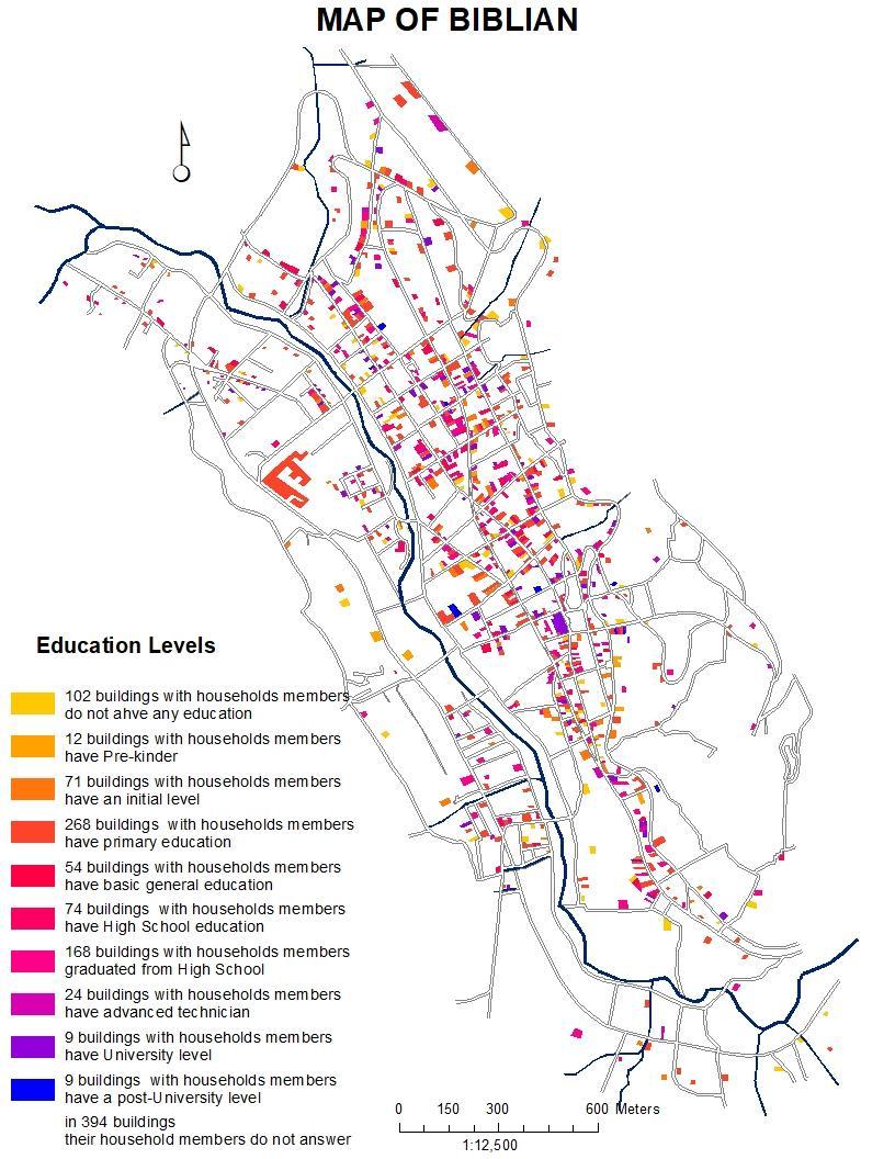Figure 4a. Variable Dependent Q22 represented in 791 buildings: Highest level of studies that reached. (Source: GIS based on updated Urban Cadaster and MIMM census of the city of Biblián in 2015)

Because it is very difficult to appreciate the information at the level of each building, these being distributed throughout the city of Biblián and separated from each other, it was necessary to first transform the polygons that represent buildings into points containing the values of the variable Q22 and then generate a spatial interpolation using the method of natural neighbors among the 791 buildings (now points, which include horizontal property) (Fig. 4b).

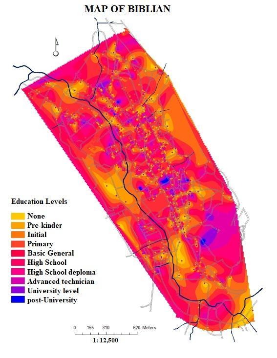Figure 4b. Spatial interpolation between 791 buildings of the Dependent Variable Q22: Highest level of studies that reached (Source: GIS based on updated urban cadaster and MIMM census of the city of Biblián in 2015)

Map 3b shows a mosaic of different cores and stripes of various colors that represent the different levels of education of people in the buildings within Biblián. Obviously and according to the data with which this spatial interpolation was made, the colors of the areas where people have primary education (in orange color) and high school diploma (in pink) have a larger area and therefore stand out visually.

Regarding the second independent variable: existence of paid work (Q50), it is deduced that of the 1,185 buildings in the city of Biblián, the homes of 1,036 of them did not answer this question (87.43%) possibly due to fear and mistrust of the pollsters and only 149 of the homes in the buildings (12.57%) answered question Q22 in the MIMM census, of the same buildings, only the people in 5 households said that they had done paid work (3.36% of the valid results), while individuals of 144 of them indicated that they had not worked (96.64%) (Fig 5a). It should be noted that perhaps this data might not be accurate since people in Biblián and other towns with high illegal migration abroad, especially to the United States, are resistant to talk about their jobs, income or remittances because they do not trust in the confidentiality of the MIMM census or they think that this information will reach the Internal Revenue Service (SRI) of Ecuador, the U.S. Consulate or maybe U.S. Citizenship and Immigration Services.

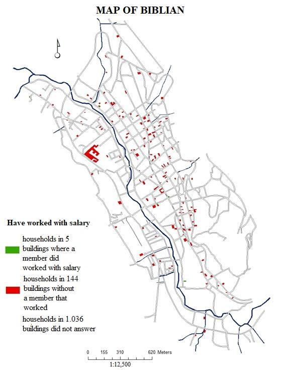Figure 5a. Dependent Variable Q50 represented in 149 buildings: have you done paid work? (Source: GIS based on updated urban cadaster and MIMM census of the city of Biblián in 2015)

In the same way that we worked with the first independent variable (Q22), we worked with variable Q50, where we also generated an isopleth map of isolines through spatial interpolation between the 149 buildings (now points) with valid answers, using the same technique: natural neighbors, to better visualize the spatial changes that paid and unpaid work generate in the city of Biblián (Fig. 5b).

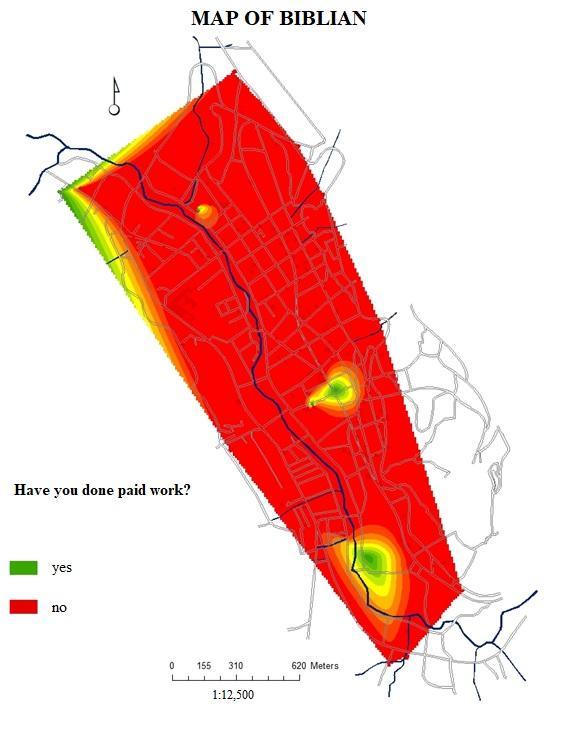Figure 5b. Spatial Interpolation between 149 buildings of the Dependent Variable Q50: Did the migrant had a paid job? (Source: GIS based on updated urban cadaster and MIMM census of the city of Biblián in 2015)

Map 5b shows only 5 cores where people have done paid work (in green), while most of the city is formed by a large area of red, the same symbolizes all buildings where its members of households do not have paid work. The reasons why this phenomenon occurs in such a large magnitude within Biblián have already explained above.

Regarding the dependent variable (number of people who have emigrated abroad for more than six months), it can be deduced that of the 1,185 buildings in the city of Biblián, the homes of 316 of them did not answer (26.67%) and only 869 of the people residing in them (73.33%) answered question Q74 in the MIMM census, of which, people in 743 buildings did not have relatives who had lived outside Ecuador for more than six consecutive months (85.50% of the existing responses), while 126 buildings had one or more members who had migrated abroad for more than six consecutive months (14.50% of the responses) (Fig. 6a). It is precisely these 126 buildings that were selected in the Biblián GIS. Based on them, the spatial regressions were performed and determined the level of influence of two independent variables: levels of education and paid work over the dependent variable: emigration abroad.

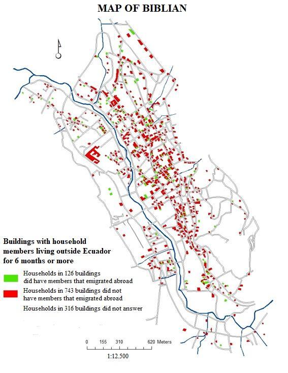Figure 6a. Dependent Variable Q74 represented in 869 buildings: You have lived outside of Ecuador for at least 6 consecutive months (Source: GIS based on updated urban cadaster and MIMM census of the city of Biblián in 2015)

As mentioned before, to better understand the behavior of emigration in the city of Biblián, we proceeded to transform the buildings (polygons) to points to generate a new spatial interpolation through the method of natural neighbors (Fig. 6b).

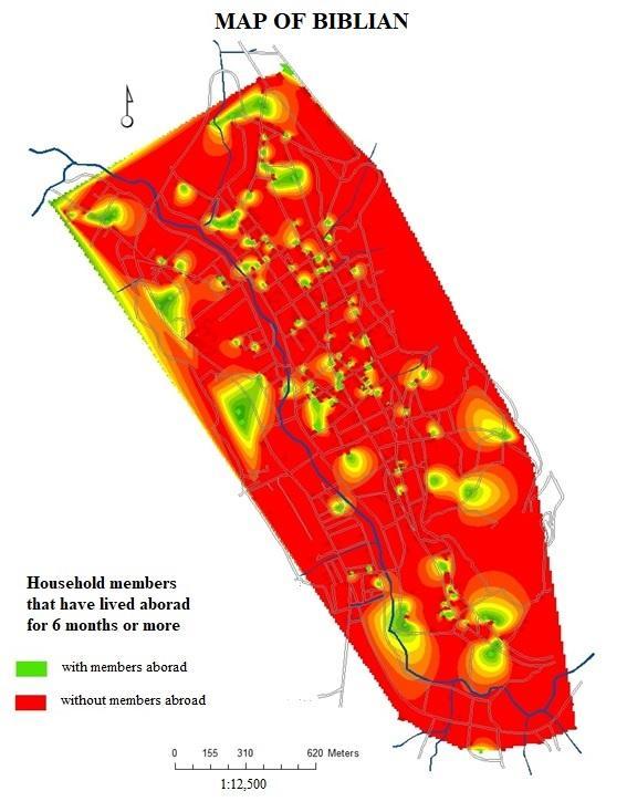Figure 6b. Spatial interpolation between 869 buildings of the Dependent Variable Q74: It has lived outside of Ecuador for at least 6 consecutive months (Source: GIS based on updated urban cadaster and MIMM census of the city of Biblián in 2015)

In map 6b it is possible to see clearly the nuclei where there are migrants for more than six months in the city of Biblián (in green); these areas are generated within a vast region of red color, the same one that represents where the members of the households have not been able to go abroad.

6.2. Results of Association Analysis through Weighted Spatial Regressions

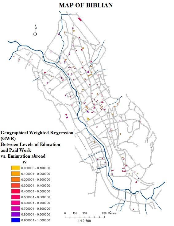
This study refers to the degree of statistical-spatial relationships between two independent variables: levels of education (question Q22 of the MIMM survey) and paid work (question Q50 of the same survey) with respect to a dependent variable, international emigration (Q74) through standard deviations or spatial distances in relation to different arithmetic means expressed in coordinates (centroids of each building).

As previously mentioned, the this technique of weighted geographical regression (GWR) was applied to the Geographical Information System of the city of Biblián based on the updated cadaster and the MIMM 2015 census data made in this city. In this particular case, it was analyzed how the 126 buildings containing different levels of education spatially influence these same 126 housing units that contain migrants abroad.

Regarding the independent variable Q22-level of education of the households only in the 126 buildings that contain people who have emigrated abroad for more than six months, the members of the households in 6 of them did not answer (4.76%), in 13 of them, people do not have any level of education (10.37%), 6 only have an initial instruction (4.76%), 49 of them said that some of their members have finished their primary education (38.89%), 8 have some level of basic general education (6.35%), 4 have reached some level of school (3.17%); in 30 buildings some members of the household have obtained a high school diploma (23.81%); in 2 housing units, its members have attended higher technical institutions (1.59%); individuals in 7 homes have a university education (5.56%) and only one person has a fourth level education, either a master's or a doctorate (0.79%).

To perform this weighted geographical regression it was necessary to change the values of the independent variable Q22, assuming that people with the lower levels of education generate a greater need to leave the country (up to a maximum of 100%), while the households with higher levels of education generate less emigration because they are the most capable to work in the local market (until it reaches minimums of 20% for postgraduate and 10% for special people). Under this assumption, the value of the 6 buildings that did not answer originally had no value, therefore they were left without data, and obviously they no longer factor into the GWR, while the initial values of 1 for none were replaced by 100. From 2 to prekinder was changed to 90, from 3 to initial was replaced by 80, from 4 to primary it was permuted by 70, from 5 to basic general it was supplanted by 60, from 7 to high school it was replaced by 50, from 8 to higher technical was changed to 40, from 9 for third level or undergraduate was replaced by 30, from 10 for fourth level or postgraduate was exchanged for 20, and the value of 11 for special education was supplanted by 10. Due to the enormous difficulty and high levels of dependency, this last group in unable to move out of the country.

Regarding the independent variable Q74, emigration abroad, the original value of the persons who had emigrated corresponded to number 1 in the MIMM census, while the value of the individuals who had not emigrated corresponded to number 2. For this reason, it retained the same value of 1 for buildings with household members that had left the country, while all buildings that did not answer this question or had not migrated abroad were eliminated from the map and consequently from the analysis of spatial regression.

The choropleth map of the GWR between the independent variable Q22 and the dependent variable Q74 shows the degree of spatial incidence that the different levels of education have on emigration abroad and are measured according to the regression coefficient (R²), and therefore, the closer the values are to 1, the higher the incidence, and to the reverse, the closer the values are to 0, the less influence will exist (Fig. 7a & 7b).

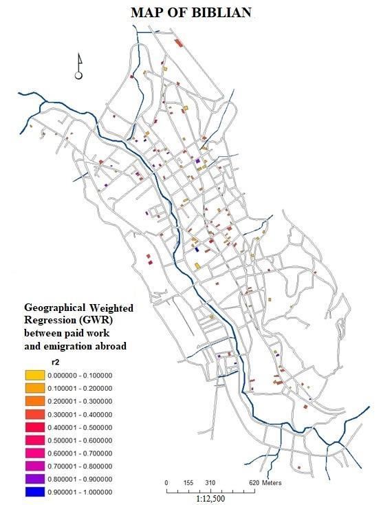
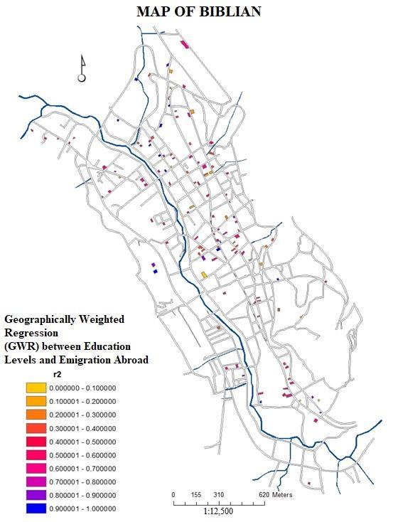Figure 7a. Spatial Regression between Levels of Education (Independent Variable Q22) and International Migration (Variable Dependent Q74) (Source: GIS based on updated urban cadaster and MIMM census of the city of Biblián in 2015)

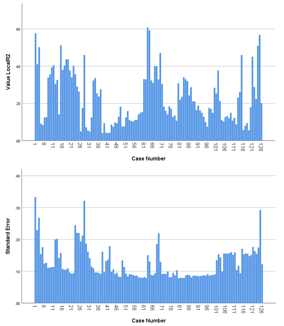
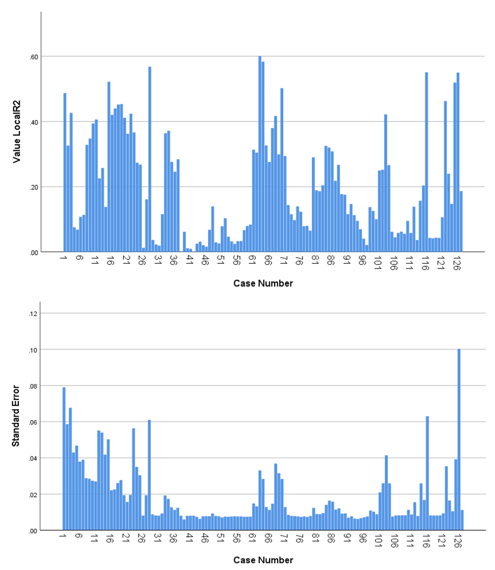Figure 7b. Histograms of R2 values and standard errors between Levels of Education (Independent Variable Q22) and International Migration (Variable Dependent Q74) in 126 buildings

In the analysis of figure 7b, great differences can be seen among R² local levels. In fact, the range varies between a minimum of R²=0.07% and maximum of R²=60.07%. Additionally, the differences in the standard errors, with a range that varies between a minimum standard error=0.60% and a maximum error=10.02% may also be noted.

Each of the polygons that represent buildings on map 6a were transformed to points to generate a spatial interpolation by the method of natural neighbors and thus better appreciate the spatial changes in a continuous surface, in addition to the values of r² or R² they were multiplied by 100 to understand the exact percentage of incidence of education levels on emigration abroad (Fig. 7c).

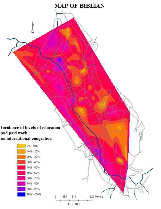
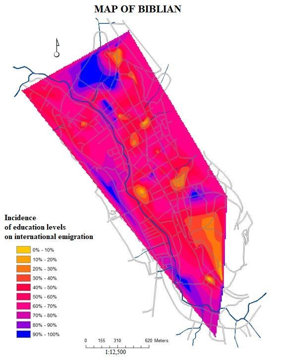Figure 7c. Spatial Interpolation of the Determination Coefficients (R2) resulting from the Spatial Regression between Levels of Education (Independent Variable Q22) and International Emigration (Dependent Variable Q74) (Source: GIS based on updated urban cadaster and MIMM census of the city of Biblián in 2015)

Analyzing map 7b, it is possible to see that there are areas where low levels of education are clearly influencing emigration abroad (blue areas): in the north of the city of Biblián there is a large nucleus and 3 small ones, in the center there is a very small one, in the south there is one of medium size, while to the east and west there are two areas of medium size. On the other hand, there are areas where low levels of education have a very slight influence on mobility abroad (yellow areas) which are distributed as follows: 6 small nuclei in the south, a small area and two medium-sized ones in the center and a large nucleus and another small one in the south of the city.

Regarding the independent variable Q50-existence of paid work of household members, in the 126 buildings that contain people who have emigrated abroad for more than six months, people in 100 of them did not answer (79.36%), in 5 of them the individuals did have work (3.97%), while in 21 buildings their members had no employment at the time of emigration (16.67%).

To perform this GWR, it was necessary to change the values of independent variable Q50, assuming that the non-existence of employment forced people to leave the country, which is why the original value of 1 in the survey was changed to 100 in the GIS; while the people who did have work in the MIMM survey had the value of 2, it was replaced by 0, under the assumption that these people have no interest in emigrating since they are safe in the workplace, while the people who did not answer in the buildings were left without any value.

The choropleth map of the weighted spatial regression between the independent variable Q50 and the dependent variable Q74 shows the degree of spatial incidence of unpaid work on emigration abroad and consists of regression coefficients (R²), just as they represent a greater influence if the values are closer to one, or vice versa, a lower incidence if the values approach to zero (Fig. 8a & 8b).

Figure 8a. Spatial Regression between unpaid or remunerated work (Independent Variable Q50) and International Emigration (Variable Dependent Q74) (Source: GIS based on updated urban cadaster and MIMM census of the city of Biblián in 2015)

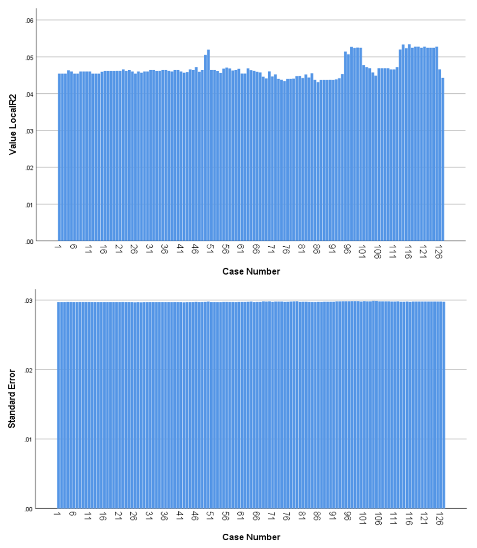Figure 8b. Histograms of R2 values and Standard Errors between unpaid or remunerated work (Independent Variable Q50) and International Emigration (Variable Dependent Q74) in 126 buildings. (Source: GIS based on updated urban cadaster and a MIMM census of the city of Biblián in 2015)

In analyzing figure 8b, it is possible to see great differences among R2 local levels, in fact the range varies between a minimum of R2=4.31% and R2=5.34%. Also, the differences are enormous among standard errors, with a range that varies between a minimum standard error=2.97% and a maximum error=2.99%.

In the same way as preceded in the previous spatial regression, in this one also each of the polygons that represent buildings in figure 8a were converted to points in order to generate spatial interpolation by the method of natural neighbors and thus allow one to be able to visualize and analyze the spatial alterations in a continuous surface of changes in the coefficients of determination which were also multiplied by 100 to understand the percentage of exact influence that exists between unpaid work and levels of emigration abroad (Fig. 8c).

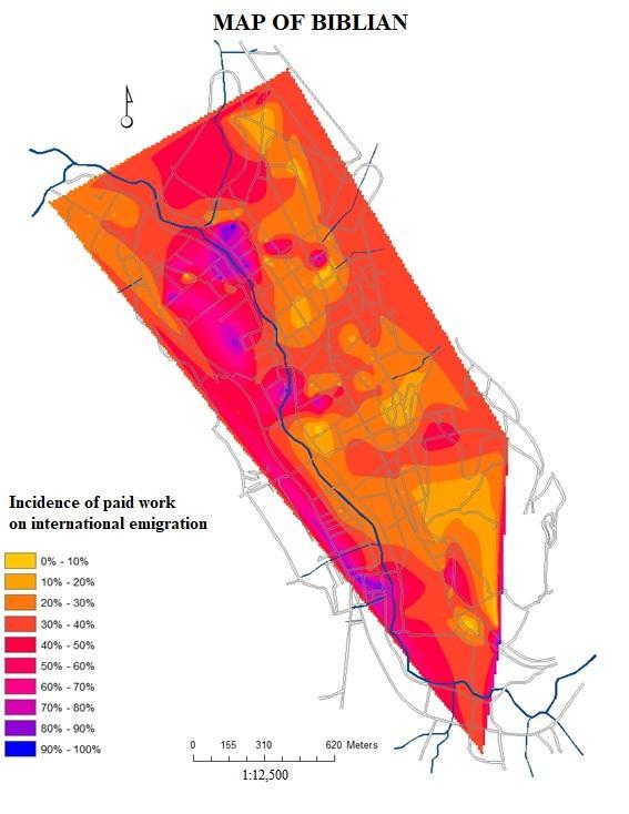Figure 8c. Spatial Interpolation of the Determination Coefficients (R2) resulting from the Spatial Regression between Paid Work (Independent Variable Q50) and International Emigration (Dependent Variable Q74) (Source: GIS based on updated urban cadaster and MIMM census of the city of Biblián in 2015)

Analyzing map 8b, it is possible to see areas where the non-existence of paid work forced people to go outdoors (in blue); in the north and southwest of the city of Biblián there are 6 small cores and one additional of medium dimensions. On the other hand, there are areas where the absence of work did not necessarily generate a process of emigration outside the country (yellow areas) which are distributed around several nuclei in the center and east of the city of Biblián.

The last spatial regression was made using the two independent variables Q22-levels of education and Q50-paid work or not, simultaneously to analyze the degree of influence they have on the independent variable Q74-emigration abroad. The same altered values were used, both Q22 and Q50, since the assumptions do not change, only the method, which in this case is a multiple spatial regression technique which produced a choropleth map showing the degree of spatial incidence that both educational levels and paid or non-paid work have together (Fig. 9a & 9b).

Figure 9a. Spatial Regression between Levels of Education (Independent Variable Q22), Paid Work (Independent Variable Q50) and International Emigration (Dependent Variable Q74) (Source: GIS based on updated urban cadaster and MIMM census of the city of Biblián in 2015)

Figure 9b. Histograms of Spatial Regression between Levels of Education (Independent Variable Q22), Paid Work (Independent Variable Q50) and International Emigration (Dependent Variable Q74) in 126 buildings (Source: GIS based on updated urban cadaster and the MIMM census of the city of Biblián in 2015)

The analysis of figure 9b indicates great differences among R2 local levels, add to that the fact that the range varies between a minimum of R2=4.02% and R2=60.76%. Also, the differences are enormous among standard errors with a range that varies between a minimum standard error of =7.85% and a maximum error of =33.32%.

Each of the buildings represented through polygons in map 8a were transformed to points in order to generate a spatial interpolation by the method of natural neighbors and thus better visualize the spatial changes in a continuous surface. In addition, the values of r² or R² were multiplied by 100 to convert them to percentages to better understand the level of incidence of education levels and of unpaid or paid work on emigration abroad (Fig. 9c).

Figure 9c. Spatial Interpolation of the Determination Coefficients (R2) resulting from the Spatial Regression between Levels of Education (Independent Variable Q22), Paid Work (Independent Variable Q50) and International Migration (Variable Dependent Q74) (Source: GIS based on updated urban cadaster and MIMM census of the city of Biblián in 2015)

Analyzing map 9b we clearly visualize areas where low levels of education and lack of adequate employment generated emigration abroad (blue areas). These nuclei are located northward and westward on the map. In addition, there are areas where higher levels of education and paid employment are lesser influencing emigration flows (yellow areas), which are represented by several nuclei, mainly in the center and eastward of the city of Biblián. The rest of the map is made up of transition zones.

7. Conclusions

The weighted geographical regressions determined which areas within the city of Biblián have the highest and lowest incidence of education and unpaid work levels in affecting international emigration. To better visualize and analyze these phenomena on continuous surfaces, spatial interpolations were applied to the variables involved in this study. The joint techniques of GWR and SI better explain associations between variables than regressions that only contain statistical data. From the analysis, we conclude that educational attainment as a proxy for joblessness, or by extension of unpaid employment in subsistence agricultural plots, is negatively correlated with emigration. This result counters the generalized idea of the brain-drain trend whereby the highly educated of the developing world--the actively working force with paid jobs-- tends to emigrate internationally towards better opportunities of employment abroad. In the case of Biblián and, by extension, most of Andean rural villages showing depopulation pressures, it is clear that the jobless are more prone to leave the area.

We determined, quite accurately, the exact location of the problems generated by emigration movements abroad (mainly to the United States) in the different areas that make up the urban extent of Biblián maintaining a geospatial memory in those who departed that makes them fund their loved ones who were left behind by way of remittances. Money sent from abroad prompted a new urban economy and facilitated the maintenance of remnant forests interspersed among the subsistance agricultural landscapes of the surrounding countryside thus maintaining a bucolic and picturesque rurality but fueled with foreign investment.

We anticipate that, in the future, the local communities will become interested in using the GWR and SI modeling scheme to identify priority areas for funding development projects. We also foresee that municipalities, provincial councils or national governments in the tropical Andes become engaged with funding and personnel to formulate policies and plans to increase the levels of education and paid employment in the zones and neighborhoods where their inhabitants have greater deficiencies of both thus contributing this research to local development and cultural affirmation and facilitating the establishment or maintenance of microrefugia for biodiversity conservation in the countryside by de-facto response to the availability of remittances that prevent further rural degradation.

ACKNOWLEDGMENTS

We are thankful to the people of Biblián and nearby country people for sharing their insights. Mario Donoso was funded by VLIR-IUC through the Program on Migration of the University of Cuenca. Fausto Sarmiento was funded by the VULPES grant ANR-15-MASC-0003 from the University of Georgia. We are indebted to Mark McCleskey who assisted with grammatical and orthographical accuracy.