-
Paper Information
- Next Paper
- Paper Submission
-
Journal Information
- About This Journal
- Editorial Board
- Current Issue
- Archive
- Author Guidelines
- Contact Us
American Journal of Geographic Information System
p-ISSN: 2163-1131 e-ISSN: 2163-114X
2019; 8(2): 55-59
doi:10.5923/j.ajgis.20190802.02

Study the Behavior of Total Least Squares Technique in Adjusting GPS Field Data - A Case Study
 Abstract
 Reference
 Full-Text PDF
 Full-text HTML
Mona S. El-Sayed
Surveying Engineering Department, Faculty of Engineering-Shoubra, Benha University, Egypt
Correspondence to: Mona S. El-Sayed, Surveying Engineering Department, Faculty of Engineering-Shoubra, Benha University, Egypt.
| Email: |  |
Copyright © 2019 The Author(s). Published by Scientific & Academic Publishing.
This work is licensed under the Creative Commons Attribution International License (CC BY).
http://creativecommons.org/licenses/by/4.0/

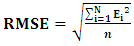
The main research fields in mathematical and satellite geodesy are computations and adjustment to assess the magnitude of errors and to study their distributions in terms of when they are within the adequate tolerance. In order to achieve this study’s objective, a GPS field direct results were adjusted using Least Squares (LS) and Total Least Squares (TLS) techniques. The difference between the LS and TLS, is that the first recognizes errors only in the observation matrix, adjusting observations in order to get the sum of their squared residuals minimum, whereas the latter acknowledge errors in both the observation matrix and design matrix, which minimizes the noise in both matrices. We used two case studies in this research, the first case study deals with baselines up to 30 km; and second one deals with baselines up to 4 km. The applied two solutions demonstrate that the result from LS technique is approximately the same of TLS on GPS network adjustment in some cases. This study main purpose is to compare the efficiency of the LS and TLS, assessing their individual accuracy and selecting the most effective method in adjusting GPS baselines. Based on statistical indicators of mean and root mean square error each model was assessed. After applying the LS and TLS techniques individually for the same data sets, it is noticed that, LS and TLS in the first case study gave root mean square error equal to 5.01mm and 5.12mm respectively. Again, in the second case study, both techniques gave the same results. Accordingly, this study highlights the efficiency of LS and TLS in solving different problems in satellite geodesy.
Keywords: Field data, GPS networks, Adjustment, Least Squares, Total Least Squares
Cite this paper: Mona S. El-Sayed, Study the Behavior of Total Least Squares Technique in Adjusting GPS Field Data - A Case Study, American Journal of Geographic Information System, Vol. 8 No. 2, 2019, pp. 55-59. doi: 10.5923/j.ajgis.20190802.02.
1. Introduction
- Least Squares (LS) is the most commonly used adjustment method in geodesy. In the recent decades it has been applied in many geodetic areas. Notable among them; approximation of the surfaces in engineering structures [1], finding the relationship between global and Cartesian coordinates [2], predictions of local coordinates [3], converting GPS data from global coordinate system to the National coordinate system [4]. Also, GPS field data is adjusted using LS like any other geodetic observations.Like any other surveying measurements, the field measurements contain errors and need to be adjusted. Adjustment is usually done using LS [5], [6], but the least squares which is based on regression analysis considers the errors in the observations matrix only [7]. As a matter of fact, errors do exist in both the design and observation matrices which must be put into consideration [5], [8], [9], [10], and [11] so, Total Least Squares technique (TLS) should be tested against LS technique.The difference between the LS and TLS, is that the first acknowledges errors only in the observation matrix and adjust observations to make the sum of their squared residuals minimum. Whereas the latter considers errors in both the observation matrix and the design matrix, which minimizes the errors in both matrices to yield a better estimate. The models used in adjusting surveying GPS networks to present this study are LS and TLS. Some studies are carried out by using TLS technique, data and perturbation size [12]. [7], [5], [14], [6], [15] have applied TLS to solve many surveying problems.
2. Methodology
- The GPS measurement method is divided into Baseline and Network model. In the Baseline method, one GPS Rover is fixed on the reference station permanently while the other rover is moving on the other ground stations to get the relative relationship between the reference station and the rest of the ground stations sequentially.While the idea of networking depends on monitoring the observation between the reference station and the rest of the stations of the network simultaneously.Differential post-processing can be divided into three segments; data analysis and validation, baseline processing, and network adjustment [16]. The data analysis and validation stage happen when the data loads into the processing software. It involves examining the data and removing any noisy data, cycle slips, and dependent baselines to improve the survey. Baseline processing is important to the post-processing method. For baseline observations, it carried out when put the GPS receiver at the base station B and the rover at the points J, K, A and L respectively. Baselines are formed by collecting carrier and phase data at two different points at the same time. By processing the baselines before adjustment, any outliers or bad points in the survey can be identified and isolated by analyzing the statistics that the baseline processor produces. The data can then be adjusted by conventional post-processing in a suitable software package which is Trimble Business Center (TBC).
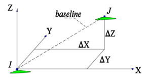 | Figure 1-a. Vector Baseline |
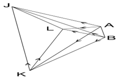 | Figure 1-b. Network |
 | (1) |
 | (2) |
 and the vector of observations
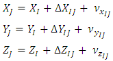
  contain the measurements of the variables a1, …am and L, respectively [5], [18]. In the classical least squares LS technique the measurements A of the variables ai (left hand side of Eq. 2) are assumed to be free of error and hence, all errors are confined to the observation vector L (the right hand side of Eq. 2), however, this assumption is frequently unrealistic sampling errors, human errors, modelling errors and instrumental errors. By solving the linear system of Eq. 2 (if m=1) with A =[a1,….., an]T and L= [l1,…ln]T.The solution of the unknown parameters X by LS approach can be achieved as denoted by Equation 2:
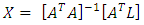 | (3) |
 | (4) |
 | (5) |
 | (6) |
 ; is the error vector of observations,
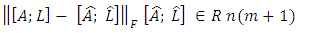
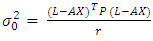
  is the error matrix of design matrix A, m is the number of unknowns and n is the number of observations. The assumption that both have separately and identically distributed rows with zero mean and equal variance. The basic TLS problem can be solved using the Singular Value Decomposition (SVD). The SVD of the augmented matrix
  can be computed according to Eq. (7)
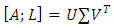 | (7) |
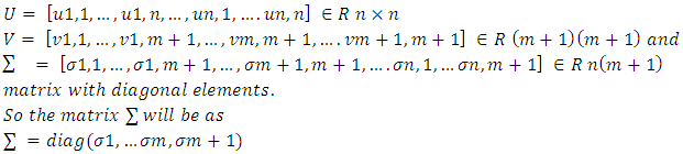 The solution of TLS is obtained after the rank reduced from (m+1) to (m) for Eq. (6).
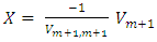 | (8) |
 | (9) |
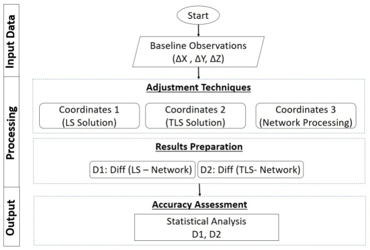 | Figure 2. Block diagram of the proposed methodology |
 | (10) |
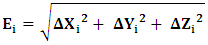
 are the residuals (the difference between the coordinates established from network adjustment and the computed one by LS and TLS) in X, Y and Z coordinates respectively.
 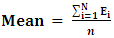 | (11) |
 | (12) |
3. Study Area
- The proposed methodology in this research is applied at two sites with different baseline ranges. Site 1 is located in Suez governorate - Egypt of area 300 km2 with baseline range up to 30 km, Site 2, which is located in Asyut governorate – Egypt of area 6 km2, has baseline separation up to 4 km. Figure (3) represents the location of the two sites.
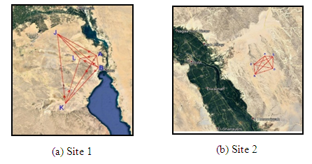 | Figure 3. Study area locations |
4. Results and Analysis
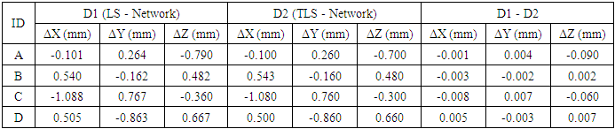
- The methodology proposed is applied on the above-mentioned solutions. The coordinates are calculated with least squares adjustment, total least squares adjustment, and network adjustment. The residuals D1 and D2 are computed at each point. Where D1 represents
 the difference between the coordinates established from network adjustment and the computed one by Least Squares (LS), and D2 represents
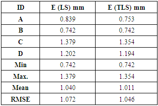
  the difference between the coordinates established from network adjustment and the computed one by Total Least Squares (TLS). The mean of absolute residuals and root mean square error are computed for the different solutions. The results of the solutions are tabulated and discussed below. Table (1) represents the results for long baselines; while Table (2) denotes the results for short baselines.
|

|
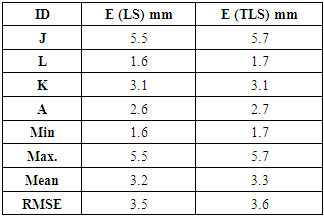
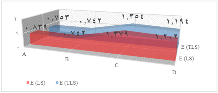
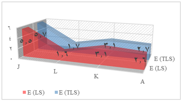 | Figure 4. Computational accuracy comparison of LS, TLS (Case Study 1) |
|
|
 | Figure 5. Computational accuracy comparison of LS, TLS(Case Study 2) |
5. Conclusions
- The research main objective is to examine the performance of total least squares with reference to least squares for both case studies to adjust the GPS networks. Through the results of the applied solutions, it can be concluded that the two techniques gave approximately the same results in two cases. The mean and RMSE of LS in the case study 1 are 4.38mm and 5.01mm respectively. The mean and RMSE of TLS in the case study 1 are 4.46m and 5.12mm respectively. Finally, the TLS technique give the same result of LS technique.