1. Introduction

The tropical forest is very important for the life of human being on the earth. It provides ecological services at the global scale [1] and plays an important role in the global carbon cycle [2, 3]. On a local scale, forests regulate water cycles and provide vegetative cover that protects the soil from erosion [4]. In the last several decades, the disturbance and loss of tropical forest have been observed in many developing countries. Forest cover has been converted to cropland, pasture and other man-made cover types in response to the humans’ demand of food, energy and other economic interests [5, 6]. This phenomenon has induced biodiversity loss, erosion and floods [7].

The North Kivu province in the Eastern part of DRC is not an exception of the deforestation phenomenon taking place in the tropical region. The DRC Ministry in charge of Environment and Nature Conservation and Tourism reported the hotspot of loss of forest cover in some regions around popular cities namely Kinshasa, Lubumbashi, Kananga, Kisangani and Kindu, as well as in the Albertin Rift (Figure 1): Province Orientale, South-Kivu and North-Kivu [8]. Except Kinshasa, the province of North Kivu had the highest annual population growth rate in DRC [9] and this number increased by more than 15% between 2010 and 2015 [10]. Hence, population increases pressure on the available forest in the region for their livelihood.

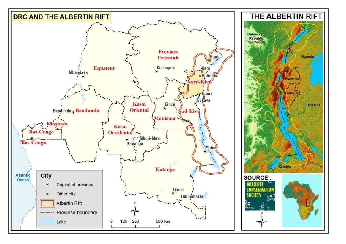Figure 1. Albertin Rift Region

Currently, an integrated approach of Remote Sensing and GIS has become an important tool in the forest assessment and monitoring [11-13]. Remote Sensing supports creating multi-spectral images and layers which are analyzed and help to produce thematic maps [14]. Since the statistical tools are integrated in GIS softwares, Remote sensing and GIS have been used in modeling key drivers of deforestation [15-18] and assess drivers between forest loss and factors associated to it such as roads [19, 20] and urban expansion [21].

This study has been therefore undertaken to estimate the forest cover loss in North Kivu province by processing Landsat images acquired in 2001 and 2015. In addition, underlying forces of deforestation have been determined using geospatial analysis tools in ArcGIS 10.3 environment. The main contribution of this study is to analyze the potential key factors driving the deforestation throughout the North-Kivu province. It includes some environmental parameters such as slope and Euclidean distance from road.

2. Study Area

2.1. Location of the Study Area

The study area the North-Kivu province located in the Eastern part of the DRC. North-Kivu is one of the provinces of DRC that extends on both sides of the Equator at latitude 0° 58’ - -2° 3’ and Eastern longitude 27° 14’ - 29° 58’ (Figure 2).

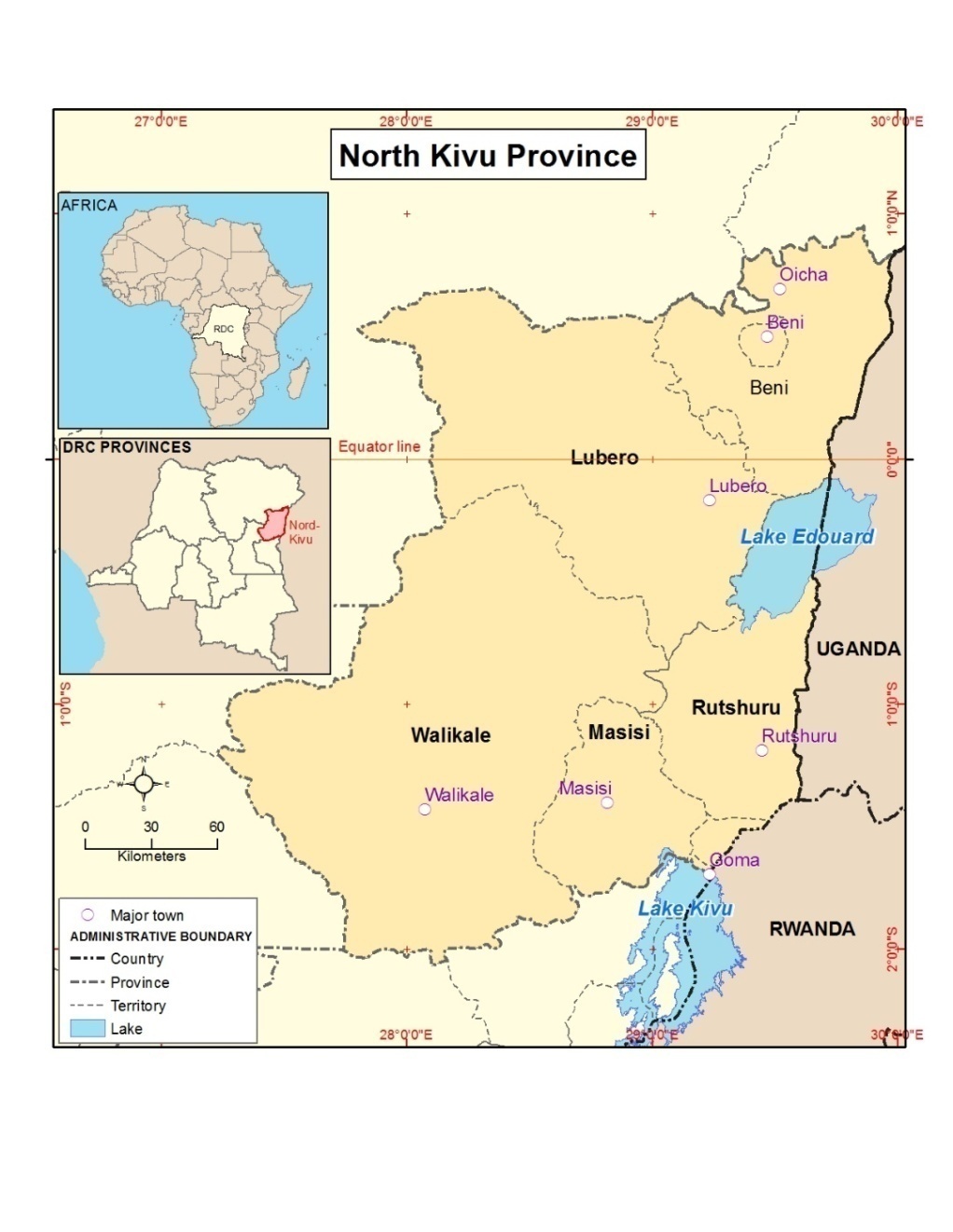Figure 2. Location map of the Nord-Kivu province

2.2. Relief and Climate of North-Kivu

The North-Kivu topography varies between 800 and 2,500 meters of altitude. However, mountains reach up to 2,500 such as mount Ruwenzori (5,119 m), volcanoes Nyamulagira volcano (3,056 m) and Nyiragongo volcano (3,470 m) [22]. The physiology of North Kivu is the result of the cracking in the Albertin Rift valley that created low and up lands from Lake Albert in North-East DRC to Lake Malawi [23].

The diversity of climate in North Kivu is a result of the heterogeneity of the topography. Below 1,000 meters the average temperature is 23°C, around 1,500 meters the temperature is near 19°C and around 2,000 m the temperature is near 15°C. The average annual rainfall varies between 1,000 mm and 2,000 mm. The lowest monthly precipitation is recorded between January and February and July and August. The North Kivu climate is characterized by four seasons: two wet seasons and two dry seasons. The first wet season appears between mid-August and mid-January and the second in mid-February to mid-July. However, the two dry seasons appear in a very short time. The first is observed between mid-January and mid-February and the second between mid-July and mid-August [22].

3. Materials and Methods

3.1. Variables

The area covered by forest in 2001 and converted into non-forest cover area in 2015 was the dependent variable used to analyze the key factors explaining the Forest Cover Loss (FL) in the province of North Kivu, DRC. According to the United Nations Food Agriculture Organization (FAO), the forest is considered as a land spanning 0.5 hectare with trees higher than 5 meters and a canopy cover more than 10 percent [24]. The Forest loss includes not only the loss of the natural forest area but also the afforested and reforested area. The potential explaining factors we analyzed are described in the Table 1. Direct factors, in case of developing countries, are the replacement of the forest area to a non-forest land due to human activities (e.g. conversion of forest area into agriculture) or to natural hazards like volcano eruption. However, the indirect drivers relate to complex interactions of social, economic, technologic, cultural and political processes that affect direct drivers to cause deforestation [25, 26].

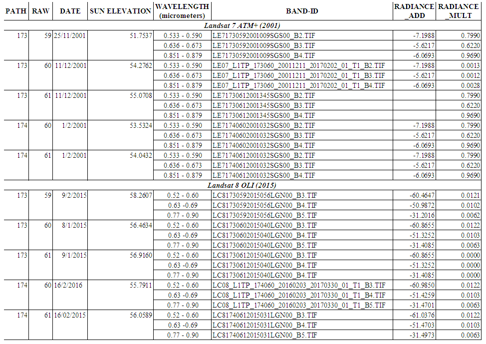Table 1. Band specifications and scalar information of used Landsat images

3.2. Data Used

This study was carried out using LANDSAT 7 ETM+ for 2001 and LANDSAT 8 OLI/TIRS for 2015 temporal images downloaded from http://earthexplorer.usgs.gov (Figure 3).

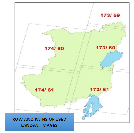Figure 3. Raw and path of Landsat images covering the Nord-Kivu province

The topography data was extracted from the Digital Elevation Model (MNT/ ASTER GLOBAL DEM) downloaded from the same website. All the Landsat images and the DEM used have 30 meters of spatial resolution. All landsat scenes with path = 174 and raw = 60 acquired in 2015 were not clear (full of cloud). Thus, the one acquired on 3 February was considered for analysis.

In addition to the above raster data used for the study, vector data of protected areas, localities, roads, rivers downloaded from the official website of the Common Geographic Reference Database: www.rgc.cd were used. This website was created by United Nations Agencies and Non-Governmental Organizations to address the mapping issue in the DRC and is managed by the DRC National Institute of Statistics. GIS layers not found in this website such as Health areas, armed groups area of influence, mining zones and Internal Displacement of population (IDP) were provided by the Information Geographic Center (CIG) and the United Nations for Stabilization of Congo (MONUSCO).

The attribute data used for some specific layers, such as population per health area and road category were provided by the Health Province Division (DPS) and the Office of Roads (OR) which are the DRC public services dealing with health and roads respectively.

3.3. Landsat Processing

The forest cover, the agriculture, the urban and the lava cover areas were derived from LANDSAT 8 OLI/TIRS and LANDSAT 7 ETM+, using the supervised multispectral classification. All used satellite images of 30 m of spatial resolution were captured during the wet season for comparison (Figure 4). The main scalar information and band specifications of used images are found in Table 1.

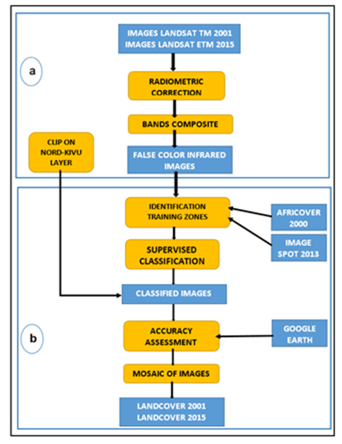Figure 4. Landsat Processing Methodology

The landsat images were processed using ArcGIS 10.3 software. The composite images of Near Infrared, Red and Green Bands were created to facilitate the extraction of the needed information such as Forest cover and the Agriculture areas. The SPOT images with a very high spatial resolution (2.5 meters) acquired in 2013 were also used as support to the interpretation keys of LANDSAT 8 OLI/TIRS as suggested by Potapov P. et al. [27]. The 2000 AFRICOVER land cover maps were also used to interpret the LANDSAT 7 ETM+.

The Atmospheric corrections were applied to remove errors and increase accuracy using the Equation 1 from Raster Calculator (Spatial Analyst) of ArcGIS 10.3 software. First, the Digital Numbers (DN) were converted to Top of Atmospheric (ToA) using the Equation 2 where DN2ToAr is Digital Numbers to Top of Atmospheric, B_Mult_B is Band specific of multiplicative bands, DN_V is Digital Numbers value and Ref-Add is Reflectance Additive. And after, the sun angle was corrected using Equation 2 where CoSun is correction for sun elevation, ToAr is Top of atmospheric reflectance and SinSunE is Sinus of sun elevation. The values used are found in the Metadata files of sets of images downloaded from the USGS website (https://earthexplorer.usgs.gov/). All band specifications and most important scalar information are found in Table 1. Bands of the scene with path-raw equal to 173-61 were not corrected owing to the lack of additive reflectance value in the metadata file.

(1)

(2)

The annual rate of deforestation was calculated using Equation 3 as recommended by Puyravaud, J. [28]. In this equation A1 and A2 represent the forest cover areas for the years t1 and t2. The deforestation rate can also be estimated in square kilometers of deforested area every year by the Equation 4 [28].

(3)

(4)

3.4. Cartographic Modelling of the Variables

The cartographic modelling of the variables from the table 2 as summarized in the Figure 5 was processed. This operation facilitated the measurement of these variables before their integration in one fishnet layer for statistic tests. A shape file of fishnet with rectangular grids of 3 km x 3km for the study area was first created. This has resulted to a total of 6812 patterns. The Raster Calculator and other tools of ArcGIS 10.3 were used in the process to produce thematic maps for the dependent and explaining variables. Figure 5 presents the workflow followed to create thematic maps of all variables used for this study.

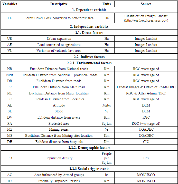Table 2. Dependent and independent variables

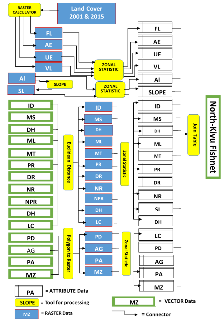Figure 5. Extraction and modeling schema of dependent and explaining variables

3.5. Statistical Analysis

3.5.1. Ordinary Least Square and Geographically Weighted Regression

Three tools were used to assess the relationship between the forest cover loss and the candidate variables. The Explanatory Regression tool was used for the model selection by generating a list of models with AICc coefficients which indicated the best model that was tested by OLS tool to detect the driving factors explaining the deforestation in the study area. The OLS regression and GWR were used to identify the key factors of deforestation and analyze their spatial heterogeneity. Subsequently, the GWR tool was also used to assess a limited key factor that can be used to predict the forest cover loss in space and time throughout the study area [29, 30].

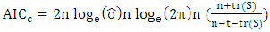
3.5.2. Calculation of Measures for Goodness-Of-Fit

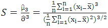
Measures of goodness-of-fit for this study aims at quantifying how well used models (Exploratory regression, OLS and GWR) fits the data and identifying the best model. A total of six main statistic tests were calculated using ArcGIS 10.3 software and interpreted. These measures include Adjusted R-Squared, Variable Inflation Factor (VIF), Jarque-Bera (JB) statistic, Moran’s Index (Moran’s I) Spatial autocorrelation, KOENKER Breusch-Pagan (BP) statistic and AIKAKE’s Information Criterion (AIC). These statistics tests helped to specify a model which meets some key requirement, i.e. the model cannot miss key explanatory variables; residuals must be normally distributed and free from spatial autocorrelation [31] to determine the passing model among two or more.

The coefficient of determination R² value, which determines how well independent variables are explaining the dependent variable, is a measure that helps to judge the performance of the model. However, a good choice for OLS and GWR models is rather based on a high Adjusted R² which is a calibration of R² value. The adjusted R² value generally increases when more independent variables are added to the model [32]. The Adjusted R² is calculated using the Equation 5 referring to the general Equation 6 for R-Squared with RSS = residual sum-of-squares, TSS = total sum-of-squares, y = response values, = fitted values, = the mean of measure values, n = sample and p = number of parameters [33].

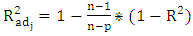(5)

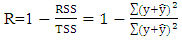(6)

The explanatory variables in a model are also expected to be free from multicollinearity. The VIF is a measure used for that and which helped in deciding which redundant variable could be removed from the model without jeopardizing it. This measure was assessed using Equation 7 where the VIF for explanatory variable j is just the reciprocal of the inverse of R² from the regression. The higher the VIF value is, the higher the collinearity is [32] which may indicate redundancy among explanatory variables [37].

(7)

Normality assumption being important in regression analysis, the JB statistic helped to test whether residuals (the observed/known dependent values minus the predicted values) follow a normal distribution. Because the model is biased if the residuals are not normally distributed (34, 35). The JB test was used to examine whether the OLS model results were trustworthy and could be used for predictions. The Equation 8 is used for calculation of the JB test, where n is the number of observations; S the sample skewness, C is sample kurtosis, and k sample estimate of the kurtosis (the number of regressors when examining residuals to an equation). 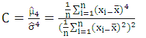The value of S and C are also defined by the mathematical Equations IX and X, where and are the estimated of the third and fourth moments respectively, is the sample mean, and is the variance. Parameters used to estimate and are found in the same equations.

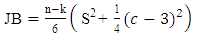(8)

(9)

(10)

Normality assumption being also important in regression models, the BP test helped to determine whether the explanatory variables had a consistent relationship to dependent variable, both in geographic and data space [34]. Considered as an asymptotical way distributed as x² with k degrees of freedom, the BP test is defined by the Equation 12 where the elements of f are defined by f_i = (e_i / s)² - 1, Z is a (n x k) matrix containing the variables thought to influence the heteroskedasticity, e is the (n x 1) vector of OLS residuals and S² the maximum likelihood variance (36).

Apart from JB and BP tests which deals with residuals in regression analysis, the Moran’s I statistic was also used to measure the degree to which residuals are spatially autocorrelated in different patterns (fishnet grids) of the study area i.e. their associated data value tended to be clustered together or dispersed in space. It is defined by the Equation 11 where is the mean of the X variable, W_ij are elements of the weight matrix and S₀ the sum of the elements of the weight matrix [37].

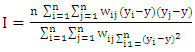(11)

To detect the best model among two or more, a statistic measure is helpful. For this study, AICc measures were calculated and used for comparing models with the same dependent variable and choosing the best model for forest cover loss prediction. The AICc value is a number that gives measures of information distance between any model which has fitted and the unknown true model [38]. The high AICc value indicates the best model and its value, as suggested by Chalton and Fotheringham [38] is calculated by Equation 13 where n is the number of observations in the dataset, is the estimate of standard deviation of the residuals, and (S) is the trace of the hat matrix.

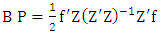(12)

(13)

3.5.3. Criteria Used for Model Selection

Based on the calculation in section 3.5.2, five criteria were considered, as suggested by Jichuan Sheng et al. [3] to assess the best models:

1) The Adjusted R-squared should be equal to or greater than 0.5 (Adjusted R² _ 0.5), which denotes that the model's goodness of fit should not be less than 0.5;

2) The p-value for regression coefficients should be no more than 0.05 (p-value _ 0.05), which suggests that the variable is statistically significant to the model;

3) The variance inflation factor value of regression variables should be no more than 7.5 (VIF _ 7.5), which ensures that there is not multicollinearity and redundant independent variables in the regression model;

4) The p-value for Jarque-Bera statistic should be greater than 0.1, which can ensure that the residuals of regression model are normally distributed. If the p-value for the Jarque-Bera statistic (test) is statistically significant, the regression model is biased and the model predictions cannot be fully trusted. When the model is biased, a key explanatory variable may be missed;

5) The p-value for spatial autocorrelation should be more than 0.1, which ensures that there is no spatial autocorrelation in the regression model based on the Moran's I value. A significant Moran's I value indicates that there is spatial autocorrelation in the model; a positive Moran's I value suggests a clustering trend, and a negative value suggests the existence of a discrete trend.

4. Results

4.1. Land Cover Change and Thematic Maps of Variables

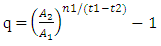
After the supervised classification of the Landsat images of the two periods (2001 and 2015), the change detection method was applied to estimate the forest cover loss, the agriculture area expansion, the urban area expansion and volcanic lava area expansion as indicated on the land cover maps (Figure 6). The overall classification accuracy was 87% following the Ground Control Points collected from Google Earth Professional application.

During the 2001 to 2015 period, the annual rate of deforestation was estimated to 1.7% using Equation 3. Moreover, we estimated to 700 square kilometers, the forest cover disappearing every year in North Kivu province (Equation 4). In some areas of the southern and northern parts of Lake Edward within the Virunga National Park, urban area has decreased in 2015 in reference to 2001 (Figure 6). This phenomenon may be explained by large evacuation operations of human population from the park initiated by the National Institute of Nature Conservation (ICCN) during 2003 and 2013 period. These operations were supported by ICCN partners and followed by some good governance measures of protected areas such as demarcation of the Virunga National Park on some parts of its border (39, 40).

Figure 6. Land cover maps of Nord-Kivu for 2001 and 2015

Figure 7 presents 21 cartographic maps modelled from the result of the Figure 5. Each map was produced using the data relating to each variable. The Dependent variable (FL) and the independent variables AE, UE and VL were extracted from data used to produce the Figure 6 while 16 other variables were extracted from data received from other sources as described in section 3.2.

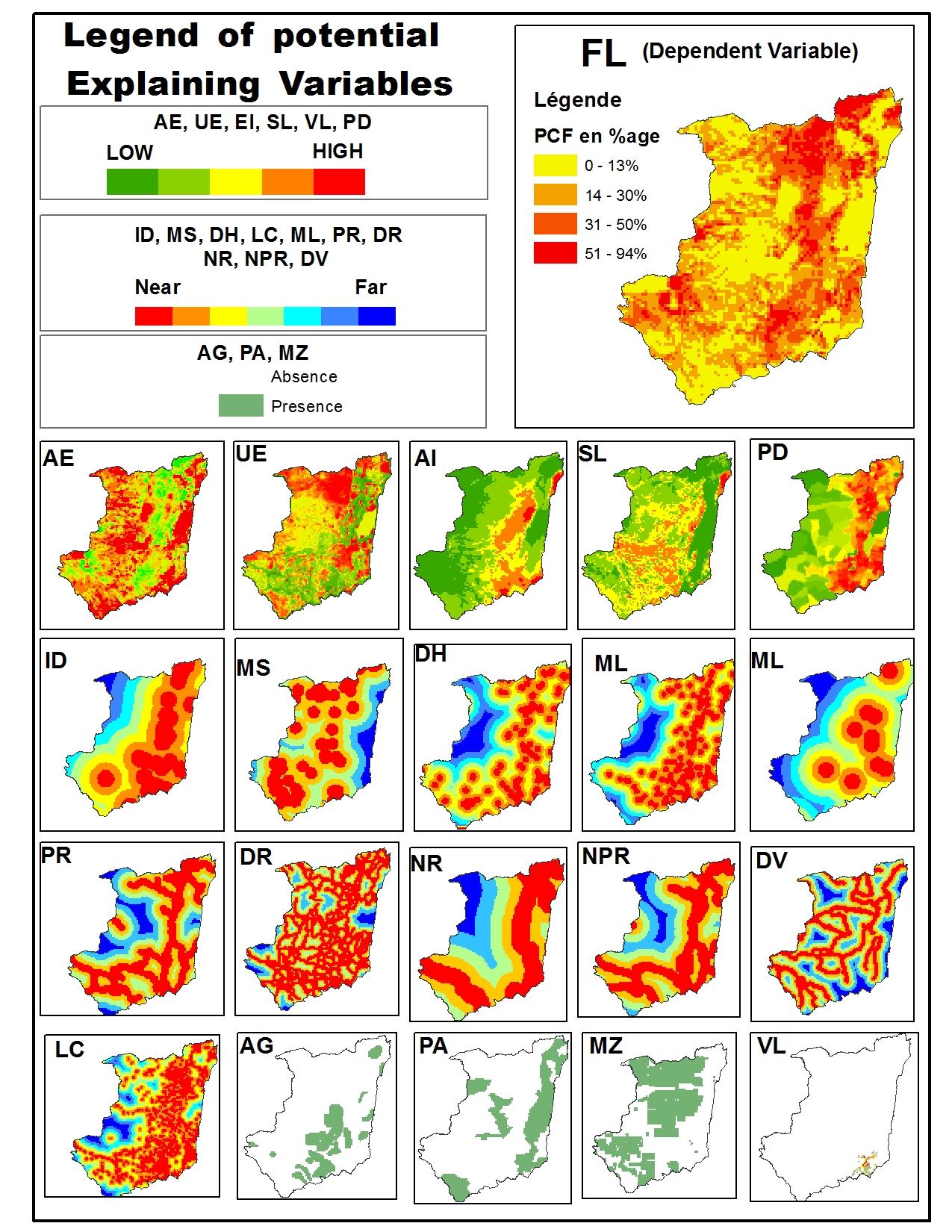Figure 7. Thematic maps of variables

4.2. Explanatory Regression Model Result

We used the exploratory regression of ArcGIS 10.3 software and came up with 17 regression models shown in the Table 3. Based on the criteria listed in the section 3.5.3, the 15^th model with the lowest AICc of 106,053 was the best fit. All these 17 models have the Adjusted R square value greater than 0.5 and a p-value for regression coefficients less than 0.05 that shows the fitness to the criteria in section 3.4.3. For all these 17 models, Jarque-Bera, Koenker (BP) and spatial autocorrelation of residuals returned a p-value of 0.000. This result was not included in Table 3 for conciseness.

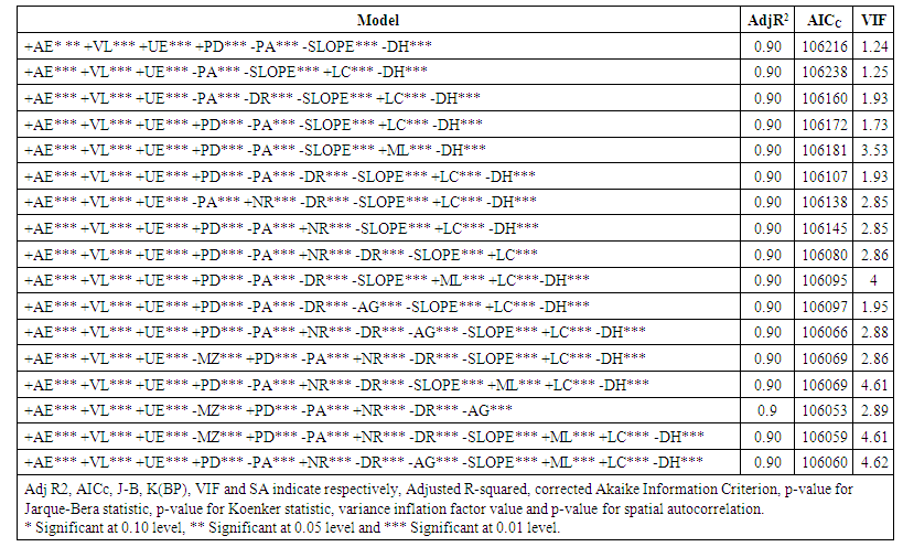Table 3. Summary of the Explanatory Regression model

The 15^th model of the Explanatory Regression proposed 12 explaining variables among a total of 20 candidates (Table 4). Consequently, the global OLS model in Table 4 tested only these 12 independent variables.

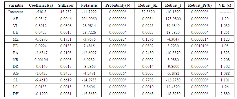Table 4. Summary of Explanatory Regression output

4.3. OLS Output Result

The global OLS linear model output of the 12 explaining variables is shown in the Table 4. After the test, the coefficients of Euclidean distance from Mining Sites (MS) and from National Road (NR) did not indicate the expected signs. This means that these unexpected coefficient signs indicate problems in the OLS model [41]. Consequently, OLS was launched for the second time without these variables and the results of the output are presented in the Table 5 including only 10 independent variables.

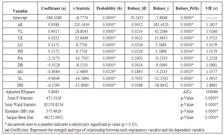Table 5. Summary of the OLS output

Relating to the model in the Table 5, the forest loss (FL) in the North Kivu province during the period starting from 2001 to 2015 was explained by the following parameters: Agriculture Expansion (AE), Volcanic lava Expansion (VL), Urban Expansion (UE), Population Density (PD), Euclidean distance from Roads (DR), Protected Area (PA), presence of Armed groups in the area (AG), Slope (SL) and Euclidean distance from hospitals (DH). The obtained global linear regression equation is: FL = 0.9386(AE) + 0.9017(VL) + 0.1172(PD) – 2.2173(PA) - 0.0128(DR) – 0.6084(AG) – 9.804922(SL) – 0.1290(DH) – 386.1089.

The OLS results in the Table 5 indicates that all the above independent variables were statistically significant at 0.05 level. The Adjusted R square value (Adj R² = 0,8946) indicated that the deforestation could be explained by the variables AE, VL, UE, PD, DR, PA, AG, SL and DH at 89%. Also, all the above variables had a Robust Probability of less than 0.01. Moreover, both the Joint F-Statistic and the Joint Wald Statistic had a P-value less than 0.01 that indicated that there is a significant linear relationship between the dependent variable and the independent variables.

Therefore, the Jarque Bera test was not statistically significant meaning that the model is unbiased.

Also, the Koenker (BP) Statistic had a statistically significant p-Value that indicate that the regression model was not stationary. This means that the regression model is not stationary and the variables have a consistent relationship in the geographic space. Consequently, the Geographically Weighted Regression (GWR) model was considered more appropriate to examine the association between the dependent variable and the explaining variables.

4.4. GWR Output Result

The result of our analysis with OLS in Table 5 confirmed that the relationship between forest cover loss and its explaining variables varies over space. So, the output of the GWR analysis examining the heterogeneous association between the variables is shown in the Table 6.

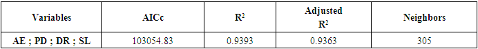Table 6. Summary of GWR output

Unlike the OLS, the GWR regression indicated four key factors explaining the forest cover loss in the North Kivu province: the Agriculture Expansion (AE), the Euclidean Distance from road (DR), the slope (SL) and the Population Density (PD). Other parameters such as VL, UE, PA, AG and DH were excluded by GWR to avoid redundancy and multicollinearity of explaining variables.

The comparative results reveal that the GWR outperformed the OLS. The GWR model has the smallest AICc (103054.83) than OLS (106086.85), and the Adjusted R-square significantly increased from 0.898 (with OLS) to 0.936 (with GWR). This indicates that 93% of the variation of the forest cover loss can be explained by only four key parameters: AE, DR, SL and PD.

5. Discussion

Among the twenty potential explaining variables tested in Table 4, ten passed with OLS regression model (Table 5) and only four passed with the GWR model (Table 6). According to the OLS regression results, there was a positive association between Forest cover loss (FL) and Agriculture expansion (AE), Volcanic lava expansion (VL), urban area expansion (UE) and the Euclidean distance from localities (LC). Our results corroborate those of Ghislain R. et al. [21] who found that Agriculture and urban expansion were the key parameters impacting forest cover loss in Panama corridor. Some other studies also revealed a positive association between the forest and the distance from roads and the density of population such as Vincent Bax et al. [20] in Amazonian Peruvian. The actor’s based survey conducted by the Ministry of Environment, Nature Conservation and Tourism (MECNT) of DRC also cited the agriculture among the key driving factors of deforestation in North Kivu [42].

The same OLS regression model results indicated a negative association with the Presence of Protected Area (PA), the Euclidean distance from roads (DR), the presence of armed groups (AG), the Slope (SL) and the Euclidean distance from hospitals (DH). The findings of Christopher P. B. et al. [19] and Van B. et al. [42] also revealed a positive association between the deforestation and the presence of protected area in Amazonian forest and DRC respectively.

Conflict may decrease or increase deforestation depending on the relationship between conflict and other causes of land use change [43]. In the North Kivu province, the population does not have access to agriculture lands in the regions influenced by local or foreign armed groups. Consequently, the forest cover in the areas influenced by armed groups had less pressure from population than secured area.

However, the Koenker (BP) statistic indicated that the OLS was not a good predictor of the forest cover loss in the North-Kivu province. This was because the independent variables vary over space. Hence, the GWR was considered as the model, which can predict better the deforestation parameters in North Kivu province as this consider the variation of the explaining factors over the geographic space.

In general, there was a positive correlation between the forest cover loss and the Agriculture expansion (AE) and the Population density (PD), and a negative correlation with the Distance from roads (DR) and the Slope (SL). This situation is due to the increase of population of North Kivu province last decades. As twenty six percent of North Kivu population rely on agriculture [44], so they need accessing to agriculture lands not far from roads and in flat areas.

Furthermore, the Figure 8 (AE) indicates that the coefficients of the Geographically Weighted Regression model for the Agriculture expansion had different values over the North Kivu province. The deeper color (blue) suggests the strong associations between the Forest cover loss and the agriculture expansion, while the lighter color (yellow) shows the week correlations. The Figure 8 (DR, PD, SL) shows the same reality for the parameters Distance from roads, Population Density and Slope.

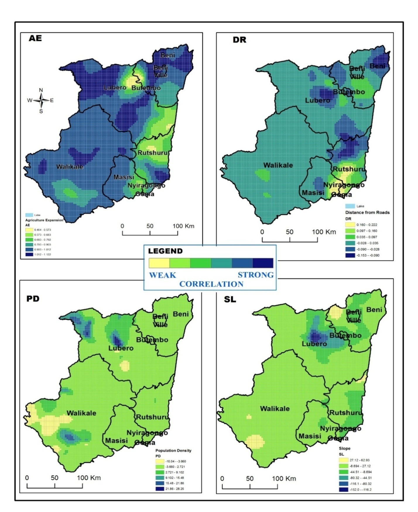Figure 8. Spatial distribution of Key factors explaining deforestation

Considering the above reality, the correlation between forest loss and agriculture expansion was strong in the western part of Lubero territory and in North of Beni territory (Figure 8.AE). The survey on deforestation causes initiated in 2012 by the DRC national Ministry of Environment and Tourism revealed agriculture as key driver of forest cover loss in Beni and Lubero territories. According to the survey report, forests have been disappearing in these territories due to shifting agriculture, perennial crop plantations and slash-and-burn agriculture [41]. In the same way, according to Figure 8 (DR), the relationship between the Forest cover loss and the distance from road was stronger in North-west of Beni territory, center of Lubero and northern part of Rutshuru than other parts of the province.

6. Conclusions

This study assessed the forest cover loss in the North Kivu province, Eastern part of DRC and analyzed its key explaining factors. The study was carried-out for the 2001 to 2015 period. A set of twenty potential independent variables were modelled and analyzed via a geospatial approach to identify the key explaining factors from them.

Using ArcGIS 10.3 software tools, results revealed an annual deforestation rate of 1.7% in the North Kivu province that equal to 700 hectares of forest cover loss every year. Both OLS and GWR regression models were tested and the GWR was estimated as the best predictive model for the Forest cover loss in the study area. The Koenker (BP) Statistic of OLS had a statistically significant p-Value (0.000*) indicating that the regression model was not stationary. Hence, there was a variation of the explaining variables in the geographic space, thus the OLS was not a good model to explain the Forest cover loss. The GWR model has the smallest AICc (103054.83) than OLS (106086.8456) and, the highest Adjusted R-square (0.9364) than the OLS (0.8984).

Using the GWR model, we identified four key factors that explained the forest cover loss in the study area. We found a positive correlation between the forest cover loss and Agriculture expansion (AE) and the Population density (PD), and a negative correlation between the Forest cover loss and the Euclidean Distance from roads and the Slope (SL).

In the last decades, the population of North Kivu province has increased while most of them rely on the agriculture for their livelihood. Accordingly, more forest cover was converted to agriculture area, especially in the regions near the roads as well as in less steep areas.

Based on our findings, we recommend the promotion of the sedentary farming in North Kivu and the prohibition of the stubble-burning and shifting agriculture. Moreover, the steep areas should be taken as priority during the afforestation and reforestation activities.

AKNOWLEDGEMENTS

Autors are thankful to the Evangelical University of Africa (UEA-Bukavu), for access to the virtual library. Special thanks to all who accepted to read this paper and provided valuable suggestions.