Mohamed I. Doma1, Rahab A. Amer2
1Assoc. Prof of Surveying and Geodesy, Civil Department, Faculty of Engineering, Menoufia University, Egypt
2GIS & Surveying Engineer, Menoufia Governorate, Egypt
Correspondence to: Mohamed I. Doma, Assoc. Prof of Surveying and Geodesy, Civil Department, Faculty of Engineering, Menoufia University, Egypt.
| Email: |  |
Copyright © 2018 The Author(s). Published by Scientific & Academic Publishing.
This work is licensed under the Creative Commons Attribution International License (CC BY).
http://creativecommons.org/licenses/by/4.0/

Abstract
Texture plays an important role in many machine vision tasks such as surface inspection, scene classification, and surface orientation and shape determination. For example, surface texture features are used in the inspection of semi-conductor wafers, gray-level distribution features of homogeneous textured regions are used in the classification of aerial imagery, and variations in texture patterns due to perspective projection are used to determine three dimensional shapes of objects. In this study, the effect of using auxiliary data in the classification results was investigated using the SVM classifier and specified training sample size, with generated Co-occurrence matrix attributes. Three investigations have been implemented: 1) using single attribute of each band. 2) Using the group attributes of each band. 3) Using the all attributes of bands and comparing the results with the case of RGB image only. The results showed that, the group of attributes of Blue band performed the best of the three bands. All classifiers are performing better using all attributes except for Neural Network. The variance attribute of the Blue and Green bands performed the best with the overall accuracy.
Keywords:
Textural Classification, SVM, GLCM, High resolution satellite imagery
Cite this paper: Mohamed I. Doma, Rahab A. Amer, Textural Attributes Classification of High Resolution Satellite Imagery, American Journal of Geographic Information System, Vol. 7 No. 5, 2018, pp. 125-132. doi: 10.5923/j.ajgis.20180705.01.
1. Introduction
Data from satellite sensors has become an important tool for researchers studying land use and land cover change. Remote sensing offers the advantage of rapid data acquisition of land use information at a lower cost than ground survey methods and the analysis of this data can provide critical insights into the evolving human environment relationship. Thematic maps derived from remotely sensed data are used in many applications, including as input parameters to models, as source of regionally extensive environmental data, or as basis of policy analysis. A variety of approaches for image classification is available and can be divided into two major groups, unsupervised and supervised. They differ in how the classification is performed [1]. In unsupervised classifications pixels are assigned to specific classes without having a prior knowledge of the classes. During an unsupervised classification process the data is aggregated into natural groups or clusters that have similar properties. In the case of supervised classification, the software system delineates specific land cover types based on statistical characterization data drawn from known examples in the image (known as training sites) [2, 3].Support vector machines (SVMs) are supervised learning algorithms based on statistical learning theory, which are considered as heuristic algorithms. The aim of the SVMs for classification is to determine a hyper-plane that optimally separates two classes. An optimum hyperplane is determined using training data and its generalization ability is verified using validation data. Thus, the primary objective of SVM is to find the optimal separating hyperplane (OSH) among all the possible hyperplanes, which is accomplished through an optimization problem utilizing Lagrange multipliers and quadratic programming methods [4]. While many hyperplanes may exist that provide effective separation, the Optimal Separating Hyperplane (OSH) minimizes classification generalization errors by maximizing the distance between itself and the planes representing the two classes.In the current study, multiclass SVM pair-wise classification strategy was applied using ENVI image processing environment. This method is based on creating a binary classifier for each possible pair of classes, choosing the class that achieved the highest probability of identification across the series pair-wise comparisons. A suitable choice of kernel allows the data to become mostly separable in the feature space despite being non-separable in the original input space.
2. Use of Textures in Image Classification
Texture is characterized by the spatial distribution of grey levels in a neighborhood. Thus, texture cannot be defined for a point. The resolution at which an image is observed determines the scale at which the texture is perceived. For example, in observing an image of a tiled floor from a large distance we observe the texture formed by the placement of tiles, but the patterns within the tiles are not perceived. When the same scene is observed from a closer distance, so that only a few tiles are within the field of view, we begin to perceive the texture formed by the placement of detailed patterns composing each tile [5, 6].For our purposes, we can define texture as repeating patterns of local variations in image intensity which is too fine to be distinguished as separate objects at the observed resolution. Thus, a connected set of pixels satisfying a given gray-level property which occurs repeatedly in an image region constitutes a textured region. A simple example is a repeated pattern of dots on a white background. Text printed on white paper such as this page also constitutes texture. Here, each gray-level primitive is formed by the connected set of pixels representing each character. The process of placing the characters on lines and placing lines in turn as elements of the page results in an ordered texture. There are three primary issues in texture analysis: texture classification, texture segmentation, and shape recovery from texture.Statistical methods are extensively used in texture classification. Properties such as gray-level co-occurrence, contrast, entropy, and homogeneity are computed from image gray levels to facilitate classification. Many texture measures have been developed [5] and have been used for image classifications [6].[7] found that textures based on a Grey-Level Co-occurrence Matrix (GLCM) and spectral features of a SPOT HRV image improved the overall classification accuracy. [8] compared GLCM, Simple Statistical Transformations (SST), and Texture Spectrum (TS) approaches with SPOT HRV data, and found that some textures derived from GLCM and SST improved urban classification accuracy. [9] investigated GLCM, Grey-Level Difference Histogram (GLDH), and Sum and Difference Histogram (SADH) textures from SPOT spectral data in an Indian urban environment, and found that a combination of texture and spectral features improved the classification accuracy. Compared to the obtained result based solely on spectral features, about 9% and 17% increases were achieved for an addition of one and two textures, respectively. They further found that contrast, entropy, variance, and inverse difference moment provided higher accuracy and the best sizes of moving window were 7 × 7 and 9 × 9. Use of multiple or multiscale texture images should be in conjunction with original spectral images to improve classification results. For a specific study, it is often difficult to identify a suitable texture because texture varies with the characteristics of the landscape under investigation and the image data used [3]. Identification of suitable textures involves determination of texture measure, image band, the size of moving window, and other parameters [10, 11]. The difficulty in identifying suitable textures and the computation cost for calculating textures limit the extensive use of textures in image classification, especially in a large area.Since texture is a spatial property, a simple one-dimensional histogram is not useful in characterizing texture (for example, an image in which pixels alternate from black to white in a checkerboard fashion will have the same histogram as an image in which the top half is black and the bottom half is white).In order to capture the spatial dependence of gray-level values which contribute to the perception of texture, a two-dimensional dependence matrix known as a gray level co-occurrence matrix is extensively used in texture analysis.
3. The Grey Level Co-occurrence Matrix
A statistical method of examining texture that considers the spatial relationship of pixels is the gray -level co-occurrence matrix (GLCM). The GLCM functions characterize the texture of an image by calculating how often pairs of pixel with specific values and in a specified spatial relationship occur in an image, creating a GLCM, and then extracting statistical measures from this matrix [7]. Gray level co-occurrence matrix (GLCM) is the basis for the Haralick texture features. This matrix is square with dimension Ng, where Ng is the number of gray levels in the image. Element [i,j] of the matrix is generated by counting the number of times a pixel with value i is adjacent to a pixel with value j and then dividing the entire matrix by the total number of such Comparisons made. Each entry is therefore considered to be the probability that a pixel with value i will be found adjacent to a pixel of value j [5]: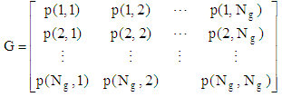 | (1) |
For a 2D image the immediate neighboring pixels can be in four different directions (0°, 45°, 90°, and 135°). For the calculation of 2D GLCM the following equation is used: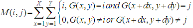 | (2) |
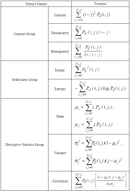
Where: i and j vary from 1 to Ng (number of grey levels).In this equation G(x, y) are the centre sample points and G(x+dx,y+dy) are the neighbouring sample points. Usually, the distance between centre and neighbouring samples is one, but greater distances can also be taken for the calculation.It is, in principal also possible to combine the four principal directions to form an average GLCM. By this approach, the spatial variations can be eliminated to a certain degree [12]. Based on the grey level co-occurrence matrix, it is possible to calculate several attributes.The first group is the contrast group and includes measurements such as contrast and homogeneity (see table 1). All the attributes from this first group are basically a function of the probability of each matrix entry and the difference of the grey levels (i and j). Therefore, these contrast group attributes are related to the distance from the GLCM diagonal.Table 1. Some texture features extracted from GLCM
 |
| |
|
Where:µi: calculates the mean based on the reference pixels, µj: calculates the mean based on the neighbour pixels,Pd (i,j): is the probability value from the GLCMσi, σj: are the standard deviations of Pd(x) and Pd(y) respectively: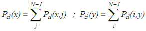 | (3) |
Values on the diagonal (where i and j are the same) result in zero contrast, whereas the contrast increases by increase of distance from the diagonal. The second attribute group is the orderliness group, which includes attributes such as energy and entropy. Attributes in the orderliness group measure how regular grey level values are distributed within a given search window. In contrast to the first group all attributes from this group are solely a function of the GLCM probability entries. The third attribute group is the statistics group, which includes attributes such as [2] measure of mean and variance. These are common mean and variance calculations applied onto the GLCM probabilities.
4. Accuracy Assessment
Meaningful and consistent reliability measures of thematic map reliability are necessary for the map user to access the appropriateness of the map data for a particular application. The accuracy of the thematic map may significantly affect the outcome of an application. Measures of map accuracy are equally important for the producer of a thematic map to analyze sources of error and weaknesses of a particular classification strategy.Measures of map accuracy are well established in the literature [13, 14]. Most commonly, accuracy assessment involves the comparison of a classified thematic map with the classification of randomly selected samples of reference data [15]. The most widely used measures of accuracy are derived from an error matrix [16]. It is worth mentioning that no one classification will be optimal from the viewpoint of each different user [17, 18]. The overall accuracy for each of the classifications was assessed using the reference data and based on equation 1: | (4) |
Where OCA is the Overall Classification Accuracy; NCP is the total Number of Correctly classified Pixels and NRP is the total Number of Reference Pixels.The kappa coefficient has many attractive features as an index of classification accuracy. In particular, it makes some compensation for chance agreement and a variance term may be calculated for it enabling the statistical testing of the significance of the difference between two coefficients [19]. This is often important, as frequently, there is a desire to compare different classifications and so matrices. To further aid this comparison, some have called for the normalization of the confusion matrix such that each row and column sums to unity [20, 21]. 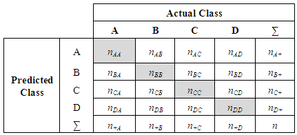 | Figure (1). The confusion matrix |
Figure 1 shows the confusion matrix, the kappa coefficient that may be derived from it. The highlighted elements represent the main diagonal of the matrix that contains the cases where the class labels depicted in the image classification and ground data set agree, whereas the off-diagonal elements contain those cases where there is a disagreement in the labels.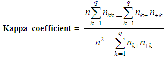 | (5) |
5. Study Area and Data Sources
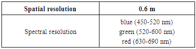
The study area chosen for this research covers approximately 520 × 270 m, and located in the western part of Luxor city, Egypt. A 0.6 meter spatial resolution and pan-sharpened image over the area of study were collected in July, 2010 by QuickBird-2 satellite (QB02) and supplied in a TIFF digital format. The image is supplied in a product level LV2A and product type standard. This image is radiometrically adjusted to improve the radiometric quality (see figure 2). Table 2 summarises the spatial and spectral characteristics of the image used (DigtalGlobe, 2006).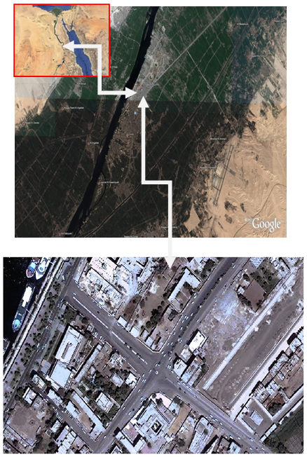 | Figure 2. The Study area (Quick bird satellite) |
Table 2. Characteristics of the image used
 |
| |
|
Additionally, field surveys were carried out using a handheld GPS to collect ground reference information. After the detailed analysis of ground reference data, it was decided that mainly six primary classes of interest covers the study area, which are: built-up areas; green areas; roads; ground; water; and platforms as shown in figure 3. 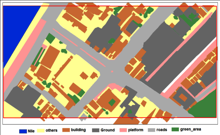 | Figure 3. The truth image |
Class “ground” mainly corresponds to grass, parking lots and bare fields. All recognizable features, independent of their size, were digitized. Buildings that were connected were digitized as individual buildings. Larger areas covered by trees were digitized as one polygon.
6. Methodology
In this study the effect of spectral attributes and textural attributes on classification results was studied using the SVM classifier. First, only the three RGB bands was tested, then a total of 27 feature attributes have been generated from the QuickBird image include the 24 attributes derived from the Grey Level Co-occurrence Matrix (GLCM). The 24 attributes derived from the GLCM were investigated at three stages: the first a contribution of single attributes, the second the group attributes of each band of the RGB bands and at last, contribution of all attributes were investigated and the results were compared with the case of RGB image only and also compared with five different supervised classifiers which are Parallelepiped, Minimum Distance, Mahalanobis Distance, Maximum Likelihood and Neural Network.
7. Results and Analysis
The RGB image was classified using SVM classifier resulted in 80% overall accuracy and kept the result to compare with the next results.
7.1. Contribution of Single Attributes
In this experiment, the main three RGB bands along with one single attribute of the 24 GLCM attributes investigated. In this regard, 24 results have been obtained as shown in Chart 1.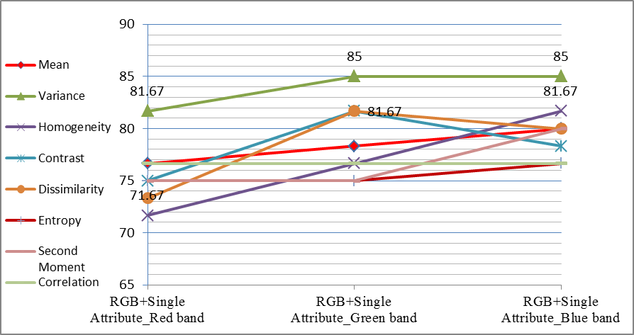 | Chart 1. The overall accuracy for SVM classifier for single attribute |
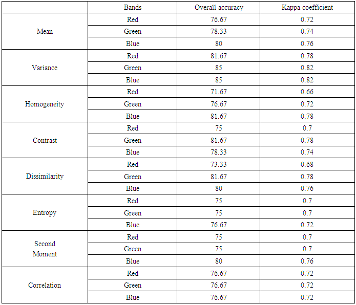
Table 3 and Chart 1 show that the variance attribute of the Blue and Green bands performed the best with overall accuracy of 85% for both, (which is higher by 5% compared with the result of SVM using only RGB image), followed by the Variance attribute of the red band, the Homogeneity attribute of Blue band, Contrast attribute of Green band and Dissimilarity attribute of Green band with 81.67% overall accuracy for all. In terms of using single attribute, the following results have been obtained: 1. The best performing attribute band is the Variance attribute for the three RGB bands.2. The worst performing attribute band is the Homogeneity attribute of the Red band.3. For Correlation attribute, the three RGB bands are equal in all values.4. The best performing attribute band for both Dissimilarity and Contrast is the Green band.5. The best performing attribute band for both Second Moment and Entropy is the Blue band, although the red and green bands have equal values.6. For the Mean and Homogeneity also the Blue band gives the best performing. Table 3. The overall accuracy and kappa coefficient for SVM classifier for single attribute in the case of proportional training size sample
 |
| |
|
7.2. Contribution of Group Attributes
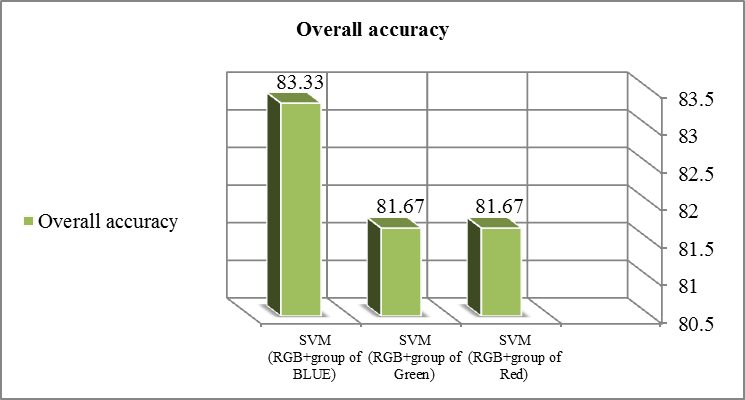 | Chart 2. The overall accuracy for SVM classifier for group of attributes in the case of proportional training size sample |
The main three RGB bands added to the group attributes of the red band once, and then to the group attributes of the green band and last to the group attributes of the blue band have been tested and evaluated. The group attributes means here mean, variance, homogeneity, contrast, dissimilarity, entropy second moment and correlation of one band. Chart 2 shows that:1. The group attributes of Blue band performed the best with overall accuracy of 83.33%. 2. The groups of the Green and Red bands perform equally with overall accuracy of 81.67%.3. These results conform to the previous results of the single attribute experiment which indicate that the group attribute of the blue band performs better than other bands with most single attributes.
7.3. Contribution of All Attributes
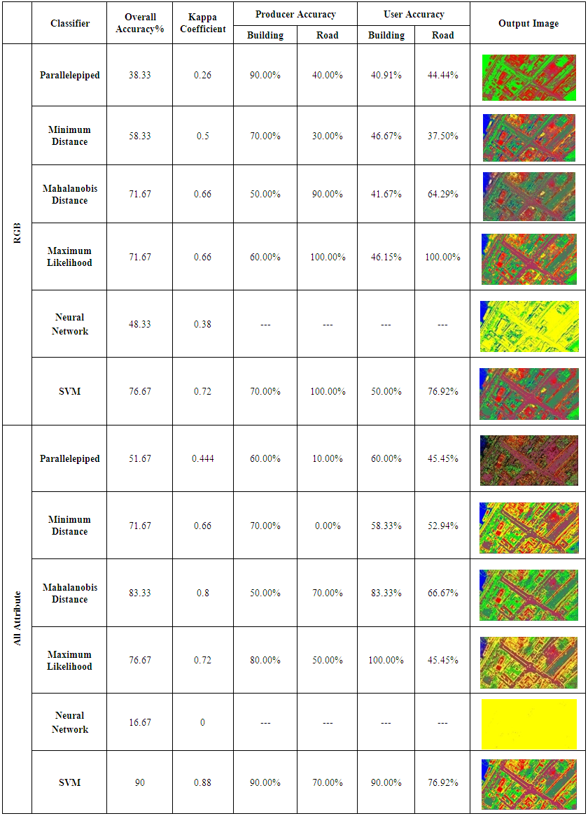
Three RGB bands added to all attributes to have a total of 27 bands have been tested and evaluated at once. In this experiment a comparison of the six supervised classifiers used in this study has been implemented, and time of processing was calculated for each classifier, see Table 4. Another comparison has been implemented using only RGB image with all attributes (RGB+24 bands of co-occurrence matrix) using six supervised classifiers, see Figure 5 and Table 5.Table 6 shows the results and outputs of the used classifiers for RGB and all attributes experiments.Chart (3), Table (5) and Table (6) show that:1. All classifiers are performing better using all attributes compared with RGB image only except for the neural network classifier which shows downward trend; it was negatively affected with the using of all attributes.2. The best performing classifiers is the SVM classifier with 90% overall accuracy and this is the optimum result followed by mahalanobis distance classifier with 83.33% overall accuracy.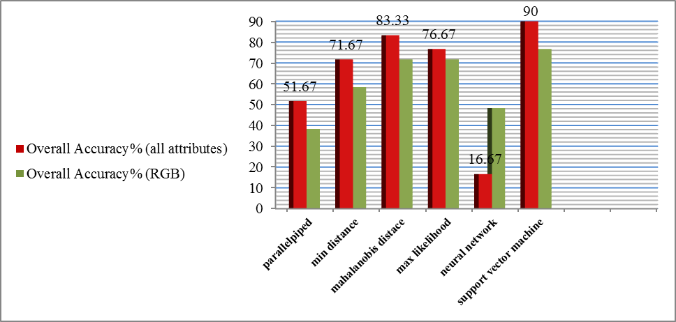 | Chart 3. Comparison of the overall accuracy using all attributes and RGB bands with supervised classifiers |
Table 4. The results and outputs of the used classifiers for RGB and all attributes experiments
 |
| |
|
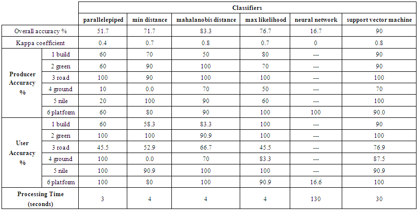 | Table 5. Classification using All Attributes+ RGB image |
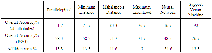
 | Table 6. The improvement in overall classification accuracy obtained for each classifier using all attributes compared with RGB image only |
8. Conclusions
The value of the map is clearly a function of the accuracy of the classification. Unfortunately, the assessment of classification accuracy is not a simple task. Accuracy assessment in remote sensing has a long and, at times, contentious history. In the current study, six supervised classification methods with different characteristics are applied to produce land use/land cover thematic map of the study area. The classifiers used in the study include: Parallelepiped, Minimum Distance, Mahalanobis Distance, Maximum Likelihood, Neural Network and Support Vector Machine (SVM). The Variance attribute of the Blue and Green bands performed the best with the overall accuracy. The attribute of the blue band performing the best with all single attributes except for both Dissimilarity and Contrast where the attribute of the Green band performing the best. The group of attributes of Blue band performed the best.
References
| [1] | Doma, M. I.; Gomaa, M. S.; Amer, R.A. (2015). Sensitivity of pixel-based classifiers to training sample size in case of high resolution satellite imagery. Journal of Geomatics, Vol. 9, No. 1, pp. 53-58. |
| [2] | Richards, J. A., Jia, X (1999). Remote Sensing Digital Image Analysis Book Ediituon 4. |
| [3] | Duda, R.O.; Hart, P.E.; Stork, D.G. (2000). Pattern Classification. 2nd Ed., Chichester, New York, John Wiley & Sons. |
| [4] | Pal, M.; Mather, P. M., (2004). Assessment of the effectiveness of support vector machines for hyperspectral data. Future Generation Computer Systems, 20(7), 1215e1225. |
| [5] | Haralick, R.M.; Shanmugam, K.; Dinstein, I. (1973). Textural features for image classification. IEEE Transactions on Systems, Man and Cybernetics, 3: 610–620. |
| [6] | Lu, D.S.; Weng, Q.H. (2007). A survey of image classification methods and techniques for improving classification performance, International Journal of Remote Sensing, 28 (5): 823–870. |
| [7] | Franklin, S.E. and Peddle, D.R., (1990). Classification of SPOT HRV imagery and texture features. International Journal of Remote Sensing, 11, pp. 551–556. |
| [8] | Gong, P.; Marceau, D.J.; Howarth, P.J. (1992). A comparison of spatial feature extraction algorithms for land-use classification with SPOT HRV data. Remote Sensing of Environment, 40: 137–151. |
| [9] | Shaban, M.A. and Dikshit, O., (2001). Improvement of classification in urban areas by the use of textural features: the case study of Lucknow city, Uttar Pradesh. International Journal of Remote Sensing, 22, pp. 565–593. |
| [10] | Franklin, S.E.; Wulder, M.A.; Lavigne, M.B. (1996). Automated derivation of geographic window sizes for remote sensing digital image texture analysis, Computers and Geosciences, 22:665–673. |
| [11] | Chen, D.; Stow, D.A.; Gong, P. (2004). Examining the effect of spatial resolution and texture window size on classification accuracy: an urban environment case. International Journal of Remote Sensing, 25:2177–2192. |
| [12] | Gao, D., (2007). Application of three-dimensional seismic texture analysis with special reference to deep-marine facies discrimination and interpretation: offshore Angola, West Africa. AAPG Bulletin 91 (12), 1665–1683. |
| [13] | Story, M.; Congalton R.G. (1986). Accuracy assessment: A user's perspective. Photogrammetric Engineering and Remote Sensing 52(3): 397-399. |
| [14] | Congalton, R.G.; Green, K. (1999). Assessing the Accuracy of Remotely Sensed Data: Principles and practices (Boca Raton, London, New York: Lewis Publishers). |
| [15] | Stehman, S. V., (1997). Selecting and interpreting measures of thematic classification accuracy. Remote sensing of Environment, 62: 77–89. |
| [16] | Foody, G.M., (2002). Status of land cover classification accuracy assessment. Remote Sensing of Environment, 80: 185–201. |
| [17] | Lark, R. M., (1995). Components of accuracy of maps with special reference to discriminant analysis on remote sensor data. International Journal of Remote Sensing, 16:1461–1480. |
| [18] | Brown, J. F.; Loveland, T. R.; Ohlen, D. O.; Zhu, Z. (1999). The global land-cover characteristics database: the user’s perspective. Photogrammetric Engineering and Remote Sensing, 65: 1069–1074. |
| [19] | Rosenfield, G. H., & Fitzpatrick-Lins, K. (1986). A coefficient of agreement as a measure of thematic classification accuracy. Photogrammetric Engineering and Remote Sensing, 52: 223–227. |
| [20] | Congalton, R.G. (1991). A review of assessing the accuracy of classifications of remotely sensed data. Remote Sensing of Environment 37: 35–46. |
| [21] | Smits, P. C.; Dellepiane, S. G.; Schowengerdt, R. A. (1999). Quality assessment of image classification algorithms for land-cover mapping: a review and proposal for a cost-based approach. International Journal of Remote Sensing, 20: 1461–1486. |

 Abstract
 Reference
 Full-Text PDF
 Full-text HTML