1. Introduction

Bathymetric information is particularly important in coastal areas which often exhibit a high population density, heavy maritime traffic. In many regions, sea depth changes because of erosion and sedimentation processes and bathymetry must often be updated. Bathymetric surveying of shallow sea water is often performed by using ships-based acoustic surveys. This technique requires heavy and expensive equipment as well as time consuming data processing [1]. Bathymetric mapping is essential for port facility management in order to avoid serious disaster. The completeness of the coastal bathymetry information is critical towards monitoring the seabed topography and detecting the emergence of new land in supporting dredging operations through prediction of navigational channel infill and estimating sediment budgets [2]. The mountains, shelves, canyons and trenches of the seafloor have been mapped with varying degrees of accuracy since the mid-nineteenth century. Today, the depth of the seafloor can be measured from kilometer- to centimetre scale using techniques as diverse as multibeam sonar from ships, optical remote sensing from aircraft and satellite, and satellite radar altimetry [3]. The measurements of water depths using sounding techniques were used for the first time by Unites States Army Corps of Engineering in 1930S. Nonetheless, it does not replace reliance on lead line depth measurement until 1950S or 1960S. Single beam-echo sounding was the most common technique that was used to measure depths. A variety of sounding techniques was used by USACE. These techniques include: single beam transducer systems, multiple transducer channel sweep systems and multi beam sweep systems. Echo sounding techniques were used for the first time in 1920S to determine the topographic of the sea floor. The initial technique was used to estimate single pulse of sound and estimate the elapsed time between the sea floor and the shipboard [4].

Bathymetric surveying of shallow water regions using echo sounding techniques was so expensive, so dangerous and slow. It took more than 200 ship-years and billions of dollars to complete the detection of sea floor topography [5]. Because of the echo methods were so limited in shallow water; bathymetry had been estimated using passive remote sensing methods in which the natural light reflecting from the sea floor is measured. Active methods were used to measure the distance to the surface using laser [6].

Shallow-water bathymetry could be determined using combined air borne LiDAR on the one hand and passive multispectral scanner (MSS) data on the other [7]. The multispectral satellite platform such as WorldView and Ikonos images are commercially available. On the other hand, the landsat-8 images are freely available. Water depths have been estimated from landsat-8 images and compared with reference hydrographic chart values. The results showed a correlation of R²=0.8951 for depths up to 10 m [8].

Several bathymetry mapping methods were used to determine the sea bed bathymetry by using remotely sensed data. The data obtained from Digital Globe Quick Bird and Landsat-7 ETM+ multispectral images were used to determine the depth of water for the Beilun Estuary, China. The data were taken at different dates and spatial resolutions. the results indicated that: 1) the tidal water line derived from near infra red (NIR) bands were the best approximation of water surface when the tidal data was absent, 2) the reflectance ratio transform model developed by [9] is a suitable method for spectral–based water depth estimation when the data in-situ was absent, 3) the error in data caused by thin clouds could be removed by fusing remote sensing images of two different sources. The correlation coefficient for the no-cloud regions was 0.74, compared to 0.26 for covered regions [10].

Remote sensing of bathymetry can be divided into two broad categories: non-imaging, and imaging methods. The non–imaging method refers to using LiDAR for mapping bathymetry. This method is able to generate accurate bathymetric information over clear water at depth up 70m. Unfortunately, this method is limited by the coarse bathymetric sampling interval and high cost. The imaging method could be implemented analytically or empirically, or by coupling both of them [11].

Several algorithms are used to classify remotely sensed images and extract data from these images such as Artificial Neural Networks (ANN), Support Vector Machines (SVMs) and Classifier Trees (CTs). ANN is one of the most common advanced classification algorithms. Classification using ANN algorithms is extremely efficient when the process of classification is not a simple one. ANN algorithms use non parametric approach so that, it become easy to incorporate supplementary data in classification process [12].

Recently, three algorithms were applied to estimate the shallow water depth at Nile Delta coastal zone, Egypt using landsat-8 image. These algorithms include: ANN, Single Band Algorithm (SBA) and Multi-Band Rotation Transform (MBRT). The results showed RMSE of 1.54m for ANN. The (SBA) model showed poor results with coefficient of determination R²=0.51. On the other hand, MBRT technique with blue and green band gave the optimum results with R² =0.80 [13].

The objective of this research is to eliminate the weaknesses resulting from the use of traditional methods. This can be achieved by using two models: MLF neural network and BE model. The probabilities from the two models are combined using FMV algorithm. The final depths can be obtained using IPWI algorithm depending on the probabilities obtained from FMV algorithm. This paper is organized as follows: section 2 describes the study area and datasets, section 3 presents the methodology while section 4 represents the results and analysis. Finally, section 5 includes the conclusions and recommendations.

2. Study Area and Data Sources

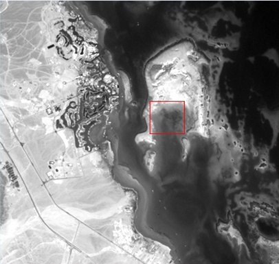
The study area is selected at El Gouna, an Egyptian resort, located 25 Kilometers (15 miles) north of Hurghada on the west coast of the Red sea in the Red sea Governorate of Egypt as shown in figure 1. Hurghada is one of the country's main tourist centers and stretches for about 36 Kilometers (22 miles) along the seashore. It is considered as the third largest city in Egypt located on the Red sea coast, after Suez and Ismailia. The study area is located between latitudes 27º21`43`` and 27º25`30``N and longitudes 33º39`03`` and 33º43`28`` E. The test area is characterized by clear and shallow waters, as well as variable depths.

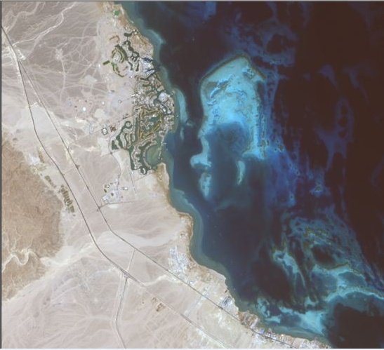Figure 1. Landsat-8 image for the study area

The Landsat-8 image of the study area is collected on 29 June 2017 and consists of 11 bands. This system uses a pushbroom sensor instead of whiskbroom sensors. It is designed with 115 miles (185 Kilometers) swath with cross-track field, and collects data from nine spectral bands; seven of them are consistent with the Thematic Mapper (TM) and Enhanced Thematic Mapper plus (ETM+) sensor. Two new spectral bands, a deep blue coastal/aerosol band and a short wave infrared cirrus band, allow scientists to estimate water quality and improve detection of high and thin clouds as shown in table 1. The provided Landsat-8 images are 12-bit radiometrically, geometrically, and terrain-corrected products.

Table 1. Landsat-8 Spectral Bands

The reference points that were used in that research were collected by echo-sounding techniques. The echo-sounding data in the study area were measured in November 2011, with survey positions being referenced to the UTM/WGS84 Zone 36N and already reduced to tidal datum. The techniques of Echo-sounding and RTK-DGPS have few characteristics as shown in table 2.

Table 2. Characteristics of Echo-sounding and RTK-DGPS

3. Methodology

The proposed method consists of several steps to derive the water depths as described in the following sections.

3.1. MLF-Based Probability

ANN are considered net-works of simple processing elements called neurons which are operating on their local data and communicated with other element [14]. There are many types of neural networks but they are similar in the basic principles [15]. Each neuron in the network consists of three layers: input layer, output layer and the hidden layer (process). MLF neural networks are considered the most popular neural network which is used in a wide variety of related problems [16]. The MLF neural network consists or neurons that are ordered in three- layers [17]: the first layer is called input layer, the second layer is called hidden layers and the last is called output layer as shown in figure 2.

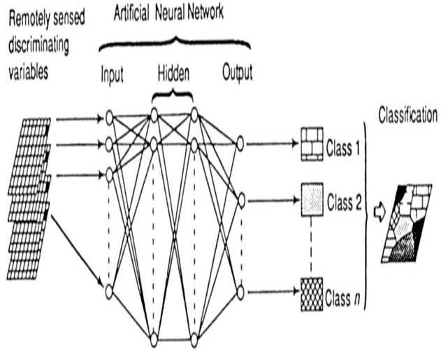Figure 2. A typical MLF with back-propagation, [18]

For training the network, MLF neural network utilizes a supervised learning technique called back-propagation training algorithm. This algorithm could be written as following in equation:

(1)

Where:

: is the activation function

: refers to the vector of weights.

x: is the vector of inputs.

b: is the bias. The activation function allows MLF networks to model nonlinear mapping well [19].

3.2. BE-Based Probability

BE algorithm is used for classification of the Landsat-8 images. A probability-based improved binary encoding algorithm (PIBE) is further introduced to match the constructed binary code to the corresponding one obtained from the training data set during the classification process. Any object in the image is translated to binary codes using the proposed PIBE. As well, the user’s requirements of the target features were quantified to binary codes. After that, the code distance was estimated based on the codes from the image. The image object was classified into land cover class with the highest similarity. BE method is considered a useful pre-processing and an efficient classifier than traditional methods for image analysis. Figure 3 shows the framework of the probability-based improved BE method which consists of two steps: 1) transfering all information into codes, 2) computing the matching probability between image objects and target classes based on the calculated distance between the corresponding binary codes [20], [21]. The image texture has shown to be important to identify the surface types in homogeneous urban regions and describes the frequency of change of image intensities [22].

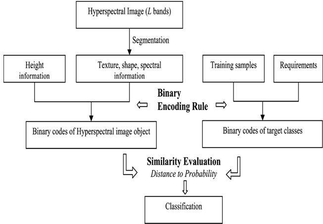Figure 3. Framework of the probability –based improved binary encoding [20]

3.3. FMV-Based Fusion of MLF and BE Results

The idea is to give some semantics or meaning to weights. Based on these semantics, the values for the weights can be provided directly. Semantics based on Fuzzy linguistic quantifiers were introduced by [23] who defined two basic types of quantifiers: absolute, and relative. Here the focus is on relative quantifiers typified by terms such as “most”, “at the least half”, or “as many as possible”. The membership function of relative quantifiers for a given pixel can be defined as [24]:

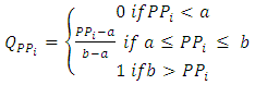(2)

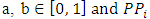Where is the class membership of the pixel as obtained for the i^th classifier. After that, [25] proposed to compute the weights based on the linguistic quantifier represented as follows:

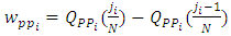(3)

Where represents the membership function of relative quantifiers as obtained for the i^th classifier, is the order of the i^th classifier after ranking for all classifiers in a descending order and N is the total number of classifiers. After that, the relative quantifier "at the least half" with the parameter pair (0, 0.5) for the membership function was applied. Depending on a particular number of classifiers N, corresponding weighting factor of the given pixel W_PP = [W_pp1,………,W_PPN ] can be obtained. Finally, (Represents the probability of FMV) can be calculated as follows:

(4)

Where is the weight based on linguistic quantifier, is the class membership of the pixel as obtained for the ith classifier, and K is the number of classes.

3.4. IPWI- Based Water Depths

IPWI is considered as the most and widely used technique that is used to estimate the depths of waters. It can be used for estimating the depth (Z) for any pixel as a function of the FMV probabilities of the known points in the training dataset. In this method, the depth of any unknown point can be estimated as follows:

(5)

Where Z is the depth of any pixel, ZP is the value of z for a pixel p, and is the probability for a point by Fuzzy Majority Voting. Figure 4 shows the illustration of the IPWI technique for estimating the depth of any point P using its combination of FMV probabilities (5%, 8%, 4%, 7%, 2%, 9%, 5%, 7%, 4%, 10%, 8%, 4%, 7%, 9%, 11%) of fifteen known depths from the data set of this research (7.279, 5.464, 10.118, 10.277, 11.478, 2.241, 5.119, 3.737, 9.995, 4.271, 3.063, 11.493, 3.804, 3.349 and 2.175) in the training dataset. By applying in equation 5, the depth of any point could be estimated.

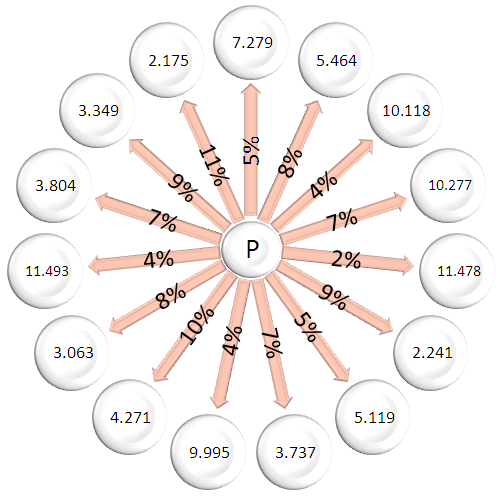Figure 4. Depth estimation using the IPWI procedure

4. Results and Analysis

4.1. Subset of Satellite Image

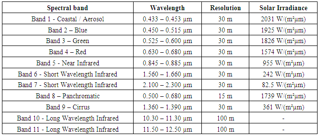
The ERDAS IMAGINE 8.4 program was used to subset the satellite images for the study area. This process was applied for the 11-bands of the satellite image using the same coordinates for the test area. ENVI 5.1 program was used to merge the 11-bands in one image. The final image that carries all bands in gray scale as shown in figure 5.

Figure 5. The merging image in gray scale

4.2. ROI (Region of Interest)

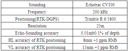
Fifteen reference points, collected using echo-sounding technique, were overlayed on the satellite image using the ENVI 5.1 program. The position of each point was determined on the image. Every depth takes a certain color in the ROI that will be used in the classification process as shown in figure 6.

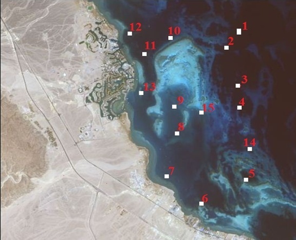Figure 6. The fifteen points or ROI overlayed on the satellite image

4.3. Classification Process

4.3.1. MLF Neural Network Classification

The supervised classification using MLF neural networks is the most popular neural networks. This classification has been performed using ENVI5.1 program for every pixel on the satellite image. After 360 iteration, the training RMS will steady at 0.2m. The results of the classification process are fifteen images. The images represent the membership value of each pixel to each point in the ROI points as shown in figure 7; from (a) through (o).

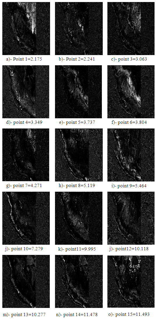Figure 7. The depth probabilities using MLF neural net work

4.3.2. BE Classification

BE is a supervised classification method that is used to classify the satellite image. ENVI 5.1 program is used to perform the BE classification after assigning the ROI. The output from the BE classification process are fifteen probability images which rpresent the memberships of each pixel to every reference height. The probability values range between 0 and 1 where; 1 indicates a complete assignment to a known depth, while 0 indicates absolute improbability.

4.4. Combining Classifiers Based on FMV

FMV has been used to combine the probabilities from the two proposed classifier (BE and MLF) with the parameter pair (0, 0.5) and using the MATLAB program. After that, the probabilities from FMV are used as input data for the IPWI to determine depths using equation 5.

4.5. IPWI-Based Water Depths

IPWI is used to estimate the water depths based on combined probability obtained by FMV images. The results of IPWI are in the form of Digital Elevation Model (DEM) as shown in figure 8.

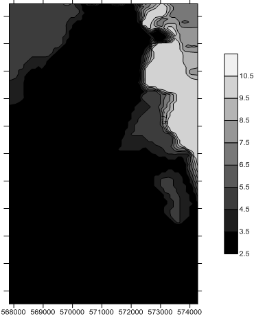Figure 8. The water depths using IPWI model

In order to evaluate the results, the minimum, maximum, mean, SD, variance and coefficient of determination (R²) were estimated and tabulated in table 3.

Table 3. Statistical analysis of the results obtained by IPWI

The coefficient of determination ranges between 0 and 1 indicating the degree of matching between the reference and model depths [26]. The low standard deviation value of 0.286m means that the difference between model depths and echo sounding data are small. The coefficient of determination (R²) was 0.877. This indicates that 87.71% of the total deferences explained by the relation between the model and reference depths, the remaining 12.29% remains unexplained. Figure 9 shows the linear correlation between the model and estimated depths.

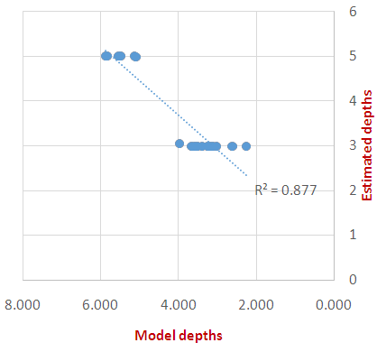Figure 9. The linear correlation between the measured and estimated depths

Once again, the estimated depths were compared with the measured depths by segmenting the depths into 2.5m range intervals as shown in figure 10. The results of IPWI are shown in colour scale range from green (2.5-5m) to red colour (>10.5m). Figure 10 shows a smooth transition from shallow water to deep water.

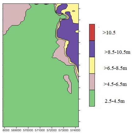Figure 10. The results of IPWI divided as five ranges

Table 4 shows smooth transition from very shallow water to shallow water. The results showed that the depths less than 4.5m have been estimated accurately with mean error of 0.44m and SD of 0.27 m, and for depths from 4.5m to 8.5m, the mean error and SD were 0.49 and 0.33m respectively. Errors are slightly greater for the depths more than 8.5m.

Table 4. Analysis of the obtained results

5. Conclusions

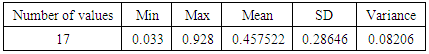
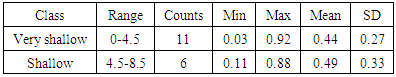
The satellite-based estimated bathymetry is an alternative method and reconnaissance tool in facilitating the increasingly demand of hydrographical surveying activities in shallow water areas. Depths of shallow water have been derived from multispectral satellite image using two models: MLF neural network and BE model. The probabilities from the two models were combined using FMV algorithm. The final depths have been obtained using IPWI algorithm depending on the probabilities obtained from FMV algorithm. The proposed method showed reasonable results with mean error of 0.457m and SD of 0.286m. Using the proposed method, the water depths of less than 4.5m can be determined accurately with mean error of 0.436m and SD of 0.265m. The errors are slightly greater for depths more than 8.5m. The coefficient of determination R² for the proposed method equals 0.877m, this was achieved between the estimated and measured depths. The proposed method can be used effectively to derive water depths with less field measurements than the conventional methods and does not require knowledge for the water attenuation. In future, different ANN models should be applied for deriving depths from multispectral satellite image with high accuracy. On the other hand, more data sources should be integrated into the system in order to derive much better results.

ACKNOWLEDGEMENTS

The authors would like to thank the data providers for their generous support.