1. Introduction

Runoff is the flowing or draining of rain water from a catchment area though a surface channel after satisfying all surface and sub-surface losses [1]. Rainstorms usually generate runoff whose occurrence and quantity is determined mainly by the distribution, duration, intensity and the characteristics of the rainfall event. Also, soil type, vegetation cover, slopes and catchment type affects the occurrence and volume of runoff.

Water harvesting, also known as water collection is a process of gathering and storing of surface runoff from a catchment area [2]. It is a common practice in arid and semi-arid regions because they act as a source of water for diverse purposes when alternative sources such as wells, springs or streams dry up [3].

The essence of estimating surface runoff is to provide important information on planning of water conservation measures, reducing the flooding hazards downstream which result in sedimentation, recharging the ground water zones, and assessment of water yield potential of the watershed. Watershed or catchment is an area covering all the land contributing runoff water to a common point known as pour point [1].

Recently, GIS and remote sensing has proved to play a vital role in runoff modelling and identification of optimal sites for water harvesting or recharging structures [4-7]. Hydrological modelling can hardly be performed without the incorporation of GIS as a tool due to its capacity to manage a large amount of spatial and attribute data [1].

Most of the work on adoption of remotely sensed data in hydrologic modelling has involved the use of SCS-CN runoff model due to its unique dependence on landcover material which is crucial when it comes to runoff [8]. The method is fast and accurate. It involves the use of a simple empirical formula and readily available tables and curves. The curve numbers are determined by the hydrologic soil group (HSG) and land use. A small curve number means little runoff and high infiltration while a high curve number implies high runoff and low infiltration.

According to Nairobi City Water and Sewerage Company (NCWSC), the city has a water deficit of approximately 200,000 cubic meters a day. It gets slightly over half a million cubic meters per day against a demand of 700,000 cubic meters. The population was projected to increase from 3.8 million in the year 2015 to 4.4 million by 2020. This explains the need to increase the supply steadily in order to evade water crisis.

Water has proved to be a vital necessity in social and economic development. The human population of Kenya and more specifically Nairobi City is ever increasing thereby raising the water demand required for domestic, industrial and other uses. However, the amount of rainfall, surface and sub-surface water sources available has either remained constant or declined over time. This has resulted in over-exploitation of these water sources hence leading to declining water table levels and water quality deterioration. Harvesting of surface runoff is hence the only untapped potential that can be utilized to salvage the situation by increasing water availability and recharging the water table in the process.

This research aimed at estimating the annual runoff potential of Northern Collector Water Tunnel (NCT) project watershed by applying Soil Conservation Service-Curve Number (SCS-CN) method using GIS. The NCT is a multibillion Kenya shilling project being implemented by the government of Kenya which is aimed at harvesting flood waters from three rivers. The water is to be supplied to Nairobi city. Questions have emerged concerning the availability of the flood waters in those rivers. It is for this reason that this research was conducted.

1.1. Literature Review

Successful planning for a precipitation harvesting system must entail determination of Runoff behavior. Early researchers on water harvesting often reported outcomes as an "annual percentage" which was pronounced as the proportion of rainfall that ran off annually [9]. However, [10] warned against the use of annual runoff percentage in the design of micro-catchment systems. [11] stated the weakness grieved by the annual runoff percentage as inability to give an indication of the relationship between rainfall intensity, runoff and duration hence limiting extrapolation to drought years or new areas.

When precipitation occurs, vegetation canopy intercept some of the falling rain and what remains thereafter falls onto the ground surface as through fall [12]. The intercepted rainwater may either evaporate or drop to the ground if rainfall proceeding is heavy and continuous. Leaf drainage and stem flow can also occur because of canopy storage capacity being exceed. This is a clear indication that the vegetation cover together with rainfall trend of a place in a way determines the quantity of rainwater losses [13]. The water lost in this process is known as interception loss. The precipitation drops that touches the soil surface can either penetrate, evapo-transpire or become stored in depressions within the ground surface. What remains after all this becomes the surface runoff [14]. It is a common occurrence after the soil saturation is achieved.

There are several methods that has been devised to quantify runoff [13, 15]. The most common approach being gauging a stream canal then measuring its water flow pattern over time. Mathematical formulas are also widely used to model the real process of runoff under normal circumstances. Physical models are hard to accomplish because most of the parameters are achieved through measurement or observation hence prone to errors and blunders. Runoff models are broadly categorised into two classes namely lumped/distributed and deterministic/ stochastic models [15, 16].

The SCS-CN approach was utilized for the accomplishment of this research. This method entails the use of an equation to make estimates of runoff depth that occurs after precipitation. The equation is empirical based and was developed in United States through observations on rainfall runoff data collected from different regions over extended duration of time [8, 14, 15]. The universal form of the SCS-CN equation according to [14] is expressed as:

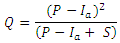(1)

Where;

Q = runoff (mm)

P = rainfall (mm)

Ia = Initial abstraction (surface storage, interception, and infiltration, mm)

S = potential maximum retention (mm)

2. Materials and Methods

2.1. The Study Area

The research focuses on the Northern Collector Water Tunnel (NCT) project which is situated within Murang’a county in central Kenya. The county resides in a total area of 2,558.8Km². NCT anticipates harnessing floodwater from three rivers shown in Figure 1 below, namely Maragua, Gikie, and Irati, which are within the same watershed with their source being Aberdare ranges forest. The area extends between latitudes 0°33'30'' S and 1°5'20'' S, and longitudes 36°41'00'' E and 37°25'20'' E. The watershed falls approximately 3,353 meters Above Sea Level (ASL) and experience extremely dissected topography which is drained by numerous rivers flowing from the Aberdare ranges to join the great River Tana.

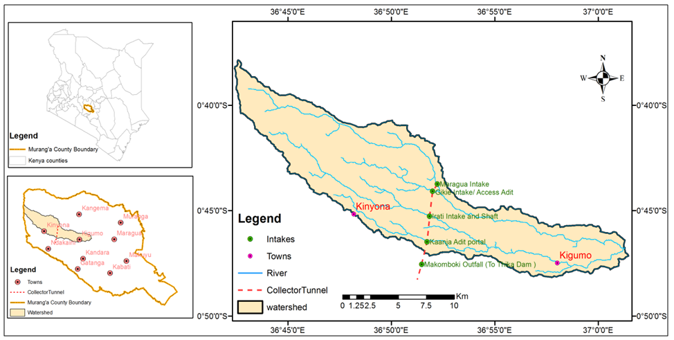Figure 1. The Study Area Map

2.2. Materials

The materials used in the study are categorized into data and software. They are summarised in the following two subsections:

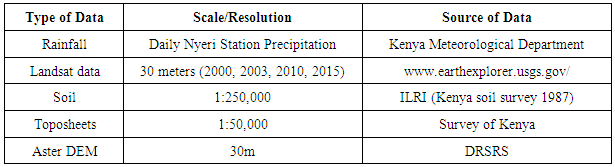
2.2.1. Data

The topographic map at the scale of 1:50000 prepared by Survey of Kenya (SoK) was utilized for delineation of rivers within the watershed and to digitize boundaries. The Landsat satellite imagery with 30m resolution downloaded from USGS website was used to prepare the land use/cover (LULC) map of the watershed. Soil data made through Kenya soil survey of 1987 on 1:50000 was utilized. 30m resolution Aster DEM data was used to generate the slope and also for determining the extents of the watershed.

Table 1. Data and their Sources

2.2.2. Software

ArcGIS 10.4 software was utilized for creating, handling and generation of different layers and maps. ERDAS Imagine 2014 was utilized in generating LULC maps due to its better accuracy in land use/cover analysis compared to other GIS software. The Geospatial Hydrologic Modelling Extension (HEC-GeoHMS) for ArcGIS was used for hydrologic modelling. Microsoft excel was utilized in mathematical computation of runoff depth from the daily rainfall data.

2.3. The Methodology

The runoff was predicted with the help of hydrological model utilizing USDA (United States Department of Agriculture) procedure for estimation of surface runoff using SCS-CN (Soil Conservation Service Curve Number) method. Flow chart in Figure 2 below summarises the methodology adopted.

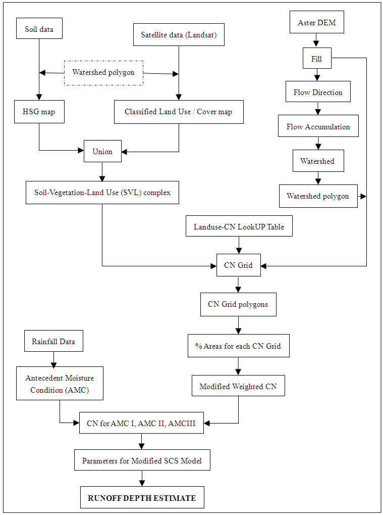Figure 2. The Methodology Flow Diagram

The process started with the delineation of the watershed extent for the three rivers using ArcGIS 10.4 software. First, the Fill hydrology tool was used to eliminate imperfection (sink) in the DEM then flow Direction tool was used to create grids representing flow direction within the cells. Flow Accumulation tool was then used to calculate the flow into each cell. The flow accumulation raster was reclassified into two classes, one with accumulation values less than 5000 and another class with values greater than 5000. The values greater than 5000 represented the stream paths which form the rivers. Pour point of the three rivers was digitized then Snap to Pour Point tool was used to establish the watershed which was later converted from raster to polygon.

The different thematic maps were prepared using ERDAS Imagine 2013 and ArcGIS 10.4. They include soil map, land use/cover classification maps and the curve number maps. Based on [14], the soil was categorized into their respective HSG while considering texture, percentage slope and infiltration rate (IR) of the soil. A field was added in the soil attribute table and the respective hydrological groups keyed in. Land use/cover classification for the years 2000, 2003, 2010 and 2015 was done in ERDAS Imagine software using unsupervised classification method with four classes namely Forest, Agriculture, Built up areas and Shrubs/Rock. K-means method of classification with between eight and sixteen classes was used then later recoded into the four classes. Accuracy assessment was then performed using ten random points per class. Aerial images were used as ground truth data during the accuracy assessment.

Soil-Vegetation-Land Use (SVL) complex was created through a vector overlay of LULC and HSG maps through a spatial Union. All polygons which did not overlay appeared with negative geometry in the attribute table and were deleted.

HEC-GeoHMS extension of ArcGIS was utilized to generate the Curve Number (CN) grid map from the fill DEM, SVL complex and CNLookUp table which are required as input datasets. The raster CN Grids generated were first converted to polygons to determine the total areas covered by specific CN. The areas obtained for the various CN were converted into a percentage of the total area of the watershed. The modified weighted curve number was calculated by multiplying all the percentage areas by their respective curve number and dividing by 100. The products of all the areas were added to give one overall weight representing the entire watershed. Since the weighted curve number value obtained was for AMC II, the assignment of AMC I and AMC III CN was done based on predefined tabulated values.

Daily precipitation data documented over time in a weather station within vicinity of the watershed was used. Daily rainfall data was chosen because the AMC of the soil can only be computed using total precipitation for five successive days preceding a storm. It is the crucial effect on the flow responses in these systems during wet weather.

To estimate the Runoff Depth, CNs were first assigned based on computed AMC that represents five-day precipitation. Potential maximum retention (S) was then computed using the equation (S = 1000/CN - 10). Subsequently, initial abstraction (surface storage, interception, and infiltration) was computed using equation (Ia = 0.2S). For all values with precipitation greater than the initial abstraction (Ia), the runoff depth was computed using equation (1), [14]. The result was daily runoff depth for all the specific days of the year.

To convert the computed runoff depth into runoff volume, the units of the depth and watershed area were first harmonised. Thereafter, the area of the watershed was multiplied with the obtained runoff depth to give the resultant volume of excess water that will pass through the pour point of the watershed after precipitation [17].

2.4. The Results

The total area of the watershed was found stretch approximately 208.3 square kilometres with its starting point at the peak of Aberdare ranges and the pour point of the three rivers being around Kigumo market within Murang’a County.

Clay soil of types montmorillonitic and kaolinitic were found to dominate the watershed as shown in Figure 3 below. The kaolinitic soil majorly concentrated on the lower parts of the watershed and comprised of types clay and silt clay textured soil falling under HSG D. Montmorillonitic soil were found to dominate the upper parts where the watershed starts and comprises of clay loam and sand clay textured soil falling under HSG C.

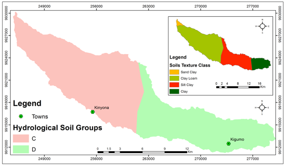Figure 3. Hydrological Soil Group (HSG) Map and Texture Classes

The Land Use Land Cover (LULC) maps and statistics (Figure 4 and Figure 6 respectively) show that forested areas occupy most parts of the watershed followed by agricultural land and built-up areas respectively. Shrubs and rocks were found to occupy the least area within the watershed. The area coverage of Shrubs and rocks remained almost the same over the entire duration of study despite small variation. Forest was found to be decreasing in size over time. There were limited changes within the conserved parts of Aberdare forest however most dynamics were occurring within the settlement areas where forested land was being cleared and converted into agricultural land as evidenced by the inverse trend of agriculture when compared with the trend of forest. Built-up area is increasing steadily though at a slower rate.

Since the watershed had two HSG and four LULC classes were considered in the study, eight curve numbers were derived as shown in the CN maps in Figure 5. The percentage areas of the different SVL complexes were then used to weight the CN under the complexes. The intention was to obtain one weighted CN representing entire watershed uniquely. The weighted Curve Number was found to increase through small values that when rounded off remains to be 84 for all the epochs as shown in Figure 7.

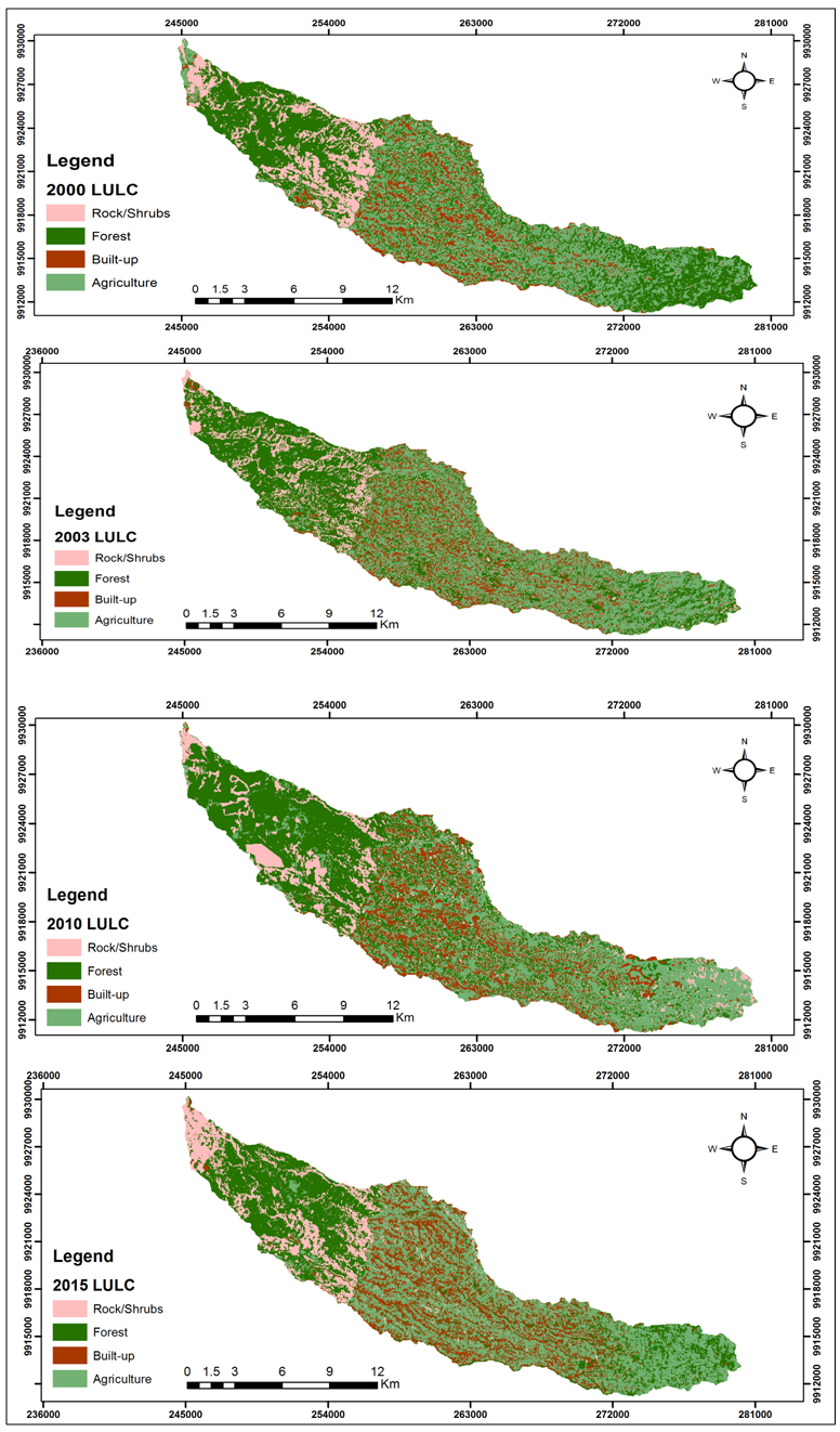Figure 4. LULC maps for the years 2000, 2003, 2010 and 2015

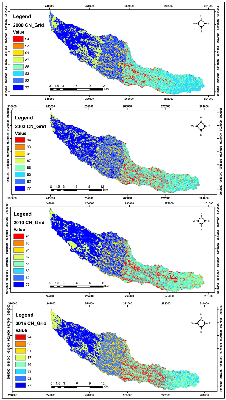Figure 5. The Curve Number maps of different SVL complexes for the four Epochs

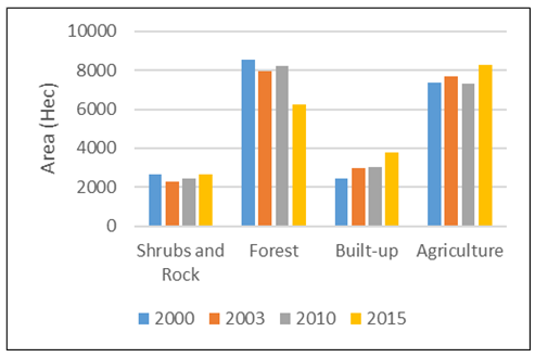Figure 6. Chart Showing Changes in LULC Trend

Figure 7. The Trend of Curve Numbers before Round off

From the runoff depth (Q) values obtained after the calculations, it is evident that the average rainfall of the area is approximately 1100mm per year which results in a runoff depth of slightly over 200mm. This implies that approximately 20% of the precipitation is converted into runoff. Precipitation that is less than 1,000mm like for the year 2000 was found to contribute the least runoff amounting to 6.07% of the total precipitation. Runoff volumes of 7,120,686 m³, 95,632,371 m³, 47,931,005 m³ and 41,848,719 m³ were obtained for the years 2000, 2003, 2010 and 2015 respectively as summarised in Table 2.

Table 2. The Summary of Runoff Depth Results

The findings were validated by comparing the values obtained with the river depth analysis result that was obtained during the research conducted at the feasibility study stage of the NCT project. From the four epochs considered, the average runoff volume obtained for the days that were found to contribute runoff was found to agree with the NCT daily runoff estimate of the river depth analysis.

2.5. Discussion of the Results

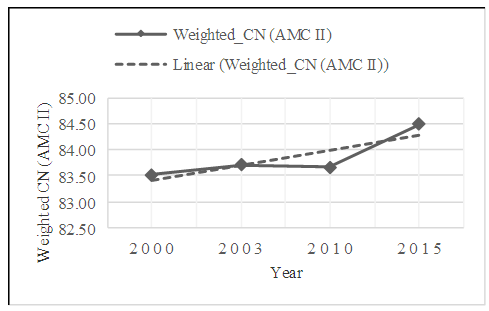
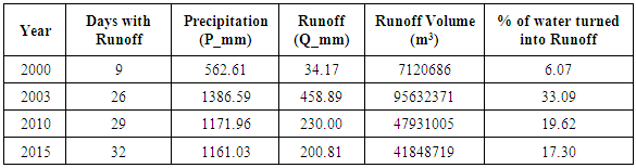
The three rivers contributing water to the collector tunnel were found to lie within one major watershed with an area of approximately 208.3 square kilometres. The tunnel cuts across the watershed tapping water from all the rivers through intakes. The flood water will be abstracted from the sub watershed before they reach the pour point of the major watershed.

From Figure 3, two HSG namely C and D were found to dominate the watershed. The soils at the northern part of the watershed were found to be of HSG C meaning they have highest runoff potential in the watershed. This is because it lies at the peak of Aberdare where rocks and mountain vegetation dominate hence limiting infiltration and favouring runoff. The southern parts of the watershed were found to be dominated by HSG D which has low runoff potential. This is majorly due to presence of agricultural lands in this section. The crops require more water hence increasing the rate of infiltration which in turn leads to lower runoff potential.

Land use/cover changes within the watershed were found to be minimal within the period of fifteen years that was considered in the study as shown in Figure 6. This was clearly evident especially with land uses that cause significant changes in runoff such us built-up areas and shrubs and rocks. The impact of these insignificant changes is reflected directly in the CN values which determine runoff potential.

Figure 7 shows the trend of the weighted CN values that were obtained from the four epochs that were studied. It is apparent that the weighted CN is increasing with time. However, the rate at which it is increasing is very low, from 83.52 in the year 2000 to 84.48 in the year 2015. When these values are rounded off, they become a weighted CN value of 84 implying that the change is so small to create a difference. This confirms that the land use/cover changes in the area has little impact on surface runoff within a span of fifteen years.

The study area was found to have high rainfall of approximately 1100mm annually (Table 2). However, it can fall below 1000mm for some drought years like in the year 2000. Despite rainfall occurring in up to one hundred days in a specific year, only thirty days in average were found to contribute water runoff amounting to approximately 20% of the total precipitation. Table 2 summarises the amount of rainfall and the resultant runoff depths.

3. Conclusions

The potential volume of annual floodwaters for the Northern Collector Water Tunnel according this this study was found to range from low values like 7,120,686 m³ (791,187 m³/day) during years with low precipitation to as high as 95,632,371 m³ (3,678,168 m³/day) during years with high precipitation (Table 2). Since the project is aimed at abstracting only 43% of the daily floodwaters which is equivalent to 513,388 m³/day, this implies that the project will still not exhaust the flood waters during dry years with lowest rainfall, like the case of the year 2003 which had the lowest runoff volume of 791,187 m³/day. This value is higher than the volume to be abstracted per day meaning some flood water will still be available to flow. This proves that areas downstream will not affected by the project.

The changes in land use/cover within the watershed focused in the study are gradual and no significant change took place within the fifteen years epoch. This is confirmed by the stagnation of weighted CN value in all epochs. From Figure 7, the value of the CNs increasing at small decimal values is a clear evidence of the limited changes that are taking place. The runoff potential is directly proportional to these changes. It can be inferred that, although the runoff within the watershed is anticipated to increase according to this finding, it will take many years before a visible change takes place.

More precipitation will result in increased surface runoff especially if it rains consecutively for many days. This is because the antecedent moisture condition (AMC) of the soil is a crucial factor determining runoff which is computed from the sum of five-day preceding precipitation. This means that rains falling for more than five consecutive days raises the AMC hence increasing the chances of more runoff.

In summary, SCS-CN method has proved to work well when localised and applied to other places outside the United States of America like this case of the Northern Collector Water Tunnel project in Kenya. The findings are comparable with the results obtained through measurement of the volumes of the rivers during dry season and wet season then estimating the runoff volumes. The application of this method can therefore be extended to other projects aiming at harvesting flood waters in Kenya and Africa at large.