1. Introduction

Urbanisation and urban growth are common phenomena throughout both the Western and the Eastern worlds. In 2014, the world’s urban population amounted to 54% of its total population. In the developed countries, 78% of the population lived in urban areas, and in the developing countries, this figure was around 52%. This indicates that currently more than half of the world’s population is urbanised (United Nations, 2014) and the present decade shows higher urban densities in the mega cities of the world, compared to the previous decades. These high urban densities occur due to one of the reasons of urban growth fuelled by migration and this is the ultimate result of urbanisation. The emergence of large cities and their rising spatial influence mark a movement of people from sprawling rural areas to predominantly urban places either in a haphazard or a planned manner. That has happened in most countries of the world over the last two centuries. This rapid and complicated urbanisation process results in the spillover of physical growth to the surrounding areas and this phenomenon is commonly referred to as ‘urban growth’. These spatial changes can be observed only over a lengthy period and the attendant physical processes show continuous spatial changes in a temporal manner. Therefore, urban growth can be considered as a spatial-temporal process. In many instances, urban growth is uncontrolled and dispersed and this is likely to impede sustainable development (Bhatta et al., 2010). A theoretical review of this spatio-temporal process leads to the conclusion that this is indeed a complex urban system, as so many scholars have observed (Kim & Batty, 2011; Cheng & Masser, 2003; Jat et al., 2008).

The urban expansion happens in three ways. Such as either with the same population density (persons per square kilometer in existing built-up areas), or with increased density, or with reduced density. Changes in the density can arise due to redevelopment of existing built-up areas at higher densities, or through infill of new developments in non-built-up areas. New development can take place adjoining the existing built-up areas or in undeveloped land that is separate from the existing built-up areas. Wilson et al. (2003) have identified above three types of urban growth, which they name as infill, edge expansion, and outlying. Mostly, outlying growth occurs in open areas and environmentally sensitive lands in and around the city. Infill growth is the main growth type and it takes place within a built-up area. Expansion growth is centred around infill growth and directly connected with existing built-up areas, whereas the outlying growth occurs separately from existing built-up areas. Outlying growth can be further divided into isolated, linear branch, and clustered branch growth. Harvey and Clark (1965) had earlier identified the three major forms of urban growth as low-density continuous development, ribbon development, and leapfrog development. These can be regarded as expansion growth, linear branch growth, and clustered (or isolated) branch growth respectively, as defined by Wilson et al. (2003). Angel et al. (2007) also identified the three basic forms of urban growth as, secondary urban centre development, ribbon development, and scattered development. In addition, physical expansion could spread along roads or development corridors, in a star shaped, linear or circular pattern, and in an orderly or disorderly manner. Quantification of these growth types is a difficult task and many scholars used GIS integrated urban analysis to quantify urban growth. Landscape matrices, Landscape Expansion Index, and urban gradient analysis are some of the major GIS based analytical tools used to quantify urban growth. Landscape matrices have some limitations for urban analysis and the other two types are effectively use for that.

1.1. Urban Gradient Analysis

Theoretically, landscape metrics were developed for measuring categorical map patterns using algorithms that quantify specific spatial characteristics in the entire landscape. It never shows spatio temporal changes. Therefore it is difficult to explore the relationships between landscape patterns and their change processes (Liu et. al., 2010). To minimize the above mentioned limitations a team of scholars (Liu et. al., 2010; Wu et. al., 2010) developed a new index, which they named as the Landscape Expansion Index (LEI). They expect to gain a better understanding of spatio-temporal land use dynamics in fast growing regions. Its value can vary depending on whether it is measured as the mean expansion index (MEI) or area-weighted mean expansion index (AWMEI). Landscape expansion index was developed for improving the results obtained from urban expansion analysis. Using LEI Liu et al. (2010) identified three growth types, namely infill growth, edge expansion, and spontaneous growth, first mentioned by Wilson et al. (2003). The analysis can be used in queries to determine which entities occur either within or outside the defined buffer zone. Hence the LEI for a new patch can be defined and calculated through examining the characteristics of its buffer zone.

“An infilling type refers to the one where the gap (or void) between old patches or within an old patch is filled up with the newly grown patch. Edge-expansion type is defined as a newly grown patch spreading unidirectionally in more or less parallel strips from an edge. If the newly grown patch is found isolated from the old, then it would be defined as an outlying type (Liu et. al., 2010).”

They introduce the following formula to calculate the LEI.

LEI - landscape expansion index

Ao - intersection between the buffer zone and the occupied category

Av - intersection between the buffer zone and the vacant category

The LEI value varies from 0 to 100. The LEI values from 1 – 50 represent infill growth, values from 51 – 100 represent edge expansion and LEI equal to zero is name as outlying growth. Liu et al. (2010) used the LEI to identify the categorised types of land expansion in an urban area of China. Similar to the above mentioned index, Wu et al. (2010) developed a new LEI for analysing agricultural lands and described three types of landscape expansion; namely infilling, edge expansion, and outlying growth. Likewise, Nong et al. (2014) used the LEI for measuring the spatio-temporal pattern of urban growth in Hanoi, Vietnam. According to the study, the LEI is classified as follows.

Lc - length of common boundary, P - perimeter of new growth area.

The value of LEI in the above study range from 0 – 1. Accordingly the urban growth types identified as follows: LEI > 0.5 = infilling growth, LEI < 0.5 = edge expansion and LEI 0 = spontaneous growth.

Although the LEI value can be used to identify the urban growth type, it never gives a meaningful picture of the spatio-temporal urban growth. Urban gradient analysis is used to minimize above gap. Here the identified growth types are further analysed using urban gradient analysis. Accordingly the different types of urban growth are analyse based on the proximity to the city using different buffer zones. This analysis helps to identify the scale of urban growth and urbanisation pattern from the city to the surroundings. In 2012, Ramachandran et al. applied gradient analysis for Greater Bangalore (now Bengaluru) to identify the urban expansion from urban to peri-urban regions. In addition 2014, Nong et al. used gradient analysis to quantify the scale and impact of urbanisation. That study create 12 buffer zones from the city, and measure LEI for each 12 buffer zones to quantify urbanisation and speed of urbanisation. Thus, the study calculated the extent of urban expansion and speed of urban expansion by using urban expansion rate and urban intensity rate. Following the above mentioned studies this research applied GIS integrated landscape Expansion Index and urban gradient analysis to measure urban growth in the Colombo district.

2. Study Area

Sri Lanka is positioned in the Indian Ocean, located very close to the Southern strip of the Indian subcontinent, lying between Northern Latitudes 5°55’ and 9°50’ and Eastern Longitudes 79°42’ and 81°52’. The land area of Sri Lanka is 65,610 sq. km., with an overall length of 432 km and, width of 224 km. Administratively Sri Lanka is divided into nine regions (or provinces) and the Western Region is the most urbanised of them. The geographical area of the Western Region covers a total extent of 369,420 ha, which comprises 5.6% of the total land area of the country. The Western Region consists of 3 districts, namely, Colombo, Kalutara, and Gampaha (Figure 1). City of Colombo is the commercial capital of Sri Lanka whereas Sri Jayewardenepura is the Administrative capital. The two cities are located in the Colombo district and urban growth occurred and expanded from those two nodal points.

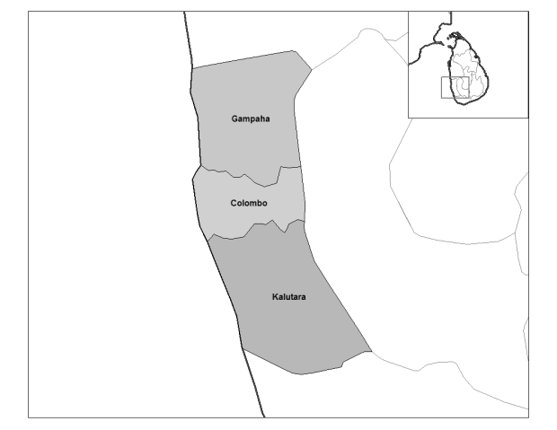Figure 1. Location of the Western Region in the Colombo District

Hence compared with the other two districts, Colombo is the most prominent, having the highest percentage of population in the region; 79.3% the Western Region’s urban population and 48.6% of the country’s urban population (Census and Statistics, 2012). Colombo district shows highest population density in the country and the figures indicate that Colombo is the most congested and urbanised district in the country as well as in the Western Region. The continuous population growth and urban growth in the Colombo District indicate a high urban density. The measurement of this pattern is complex due to its uneven growth spread. GIS based land use expansion index and gradient analysis are successfully used to quantify urban growth and this research used those techniques.

3. Data and Method

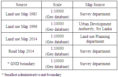
There are several sources of data used for this research and details are shown in Table 1.

Table 1. Data and data Sources

3.1. Data Classification

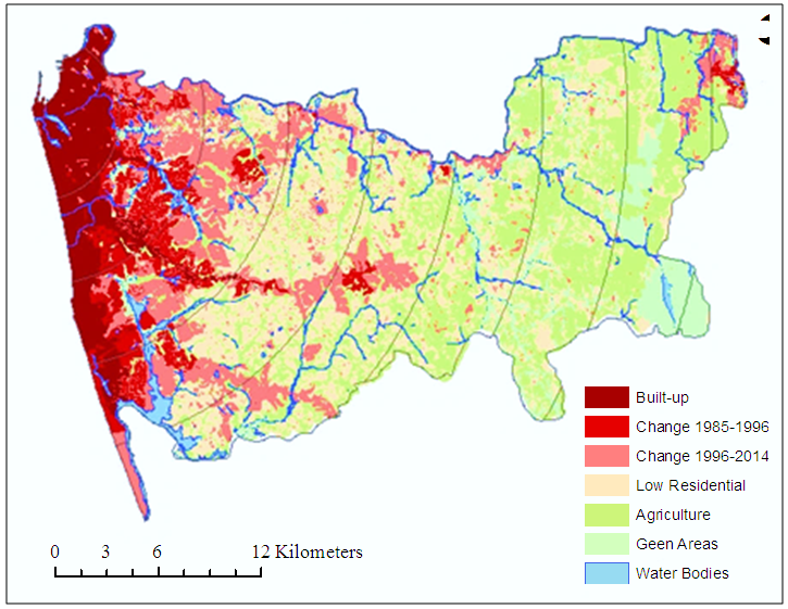
This research considered urban growth from 1980’s to 2014. The land use maps for the specified time spans (10 years each) were not available. In 1985, the Survey Department prepared a detailed land use map and again it was updated in 1996. After that in 2014, it was again updated by the land use-planning department. These three maps (1985, 1996 and 2014) were used for analysis. All Land use maps consist of 26 land use categories. Those categories reclassified into five categories; (Figure 2). Urban built up Low Residential, Agriculture, green areas, and water bodies.

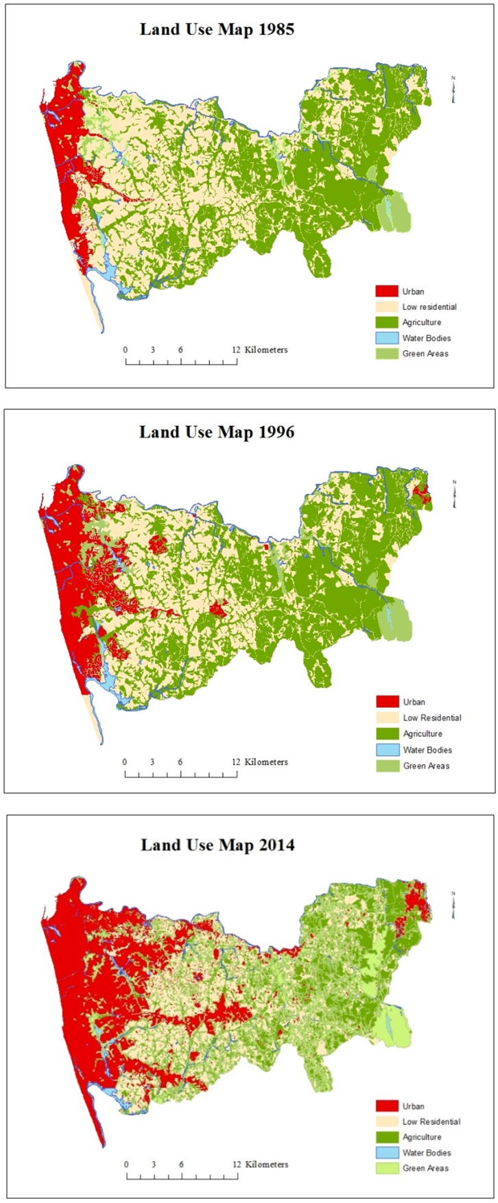Figure 2. Colombo District Land use 1985, 1996 and 2014

The research paid special attention to urban built up category because Sri Lanka does has no proper official urban classification. Therefore, the following steps were used to clarify urban area. The 1985 land use map mentioned a land use category named ‘urban built-up’, and this was considered as the base map to mark urban built-up.

1. Based on the 1985 map, the Urban Development Authority (UDA) prepared an updated version of the land use map in 1996, and it was used for the study.

2. In 2014, the land use planning department once again updated this land use map and the study referred to it as well. However, in that map too, clear urban built-up category was not included. Presently, the land uses of Colombo District are so complicated that two methods namely, method ‘a’ for MCs and UCs, and method ‘b’ for Pradeshiya Sabhas, are used to define urban built-up areas.

a). Godschalk (1988) adapted Anderson’s land use (man-made) and land cover (natural or semi-natural) classification system was used to mark out the urban built-up areas within the municipal and urban council areas of the Colombo District.

b). The Pradeshiya Sabha Act of 1987, No 15 defined 'built-up' areas, mainly with the objective of marking them out for property tax purposes. New 'built-up' areas are declared by the Minister of Local Government from time to time. Above mentioned built-up areas are also considered as part of the urban landscape.

3. Apart from the above mentioned a) and b), population density and building density were also considered as additional factors. While based mainly on the above densities, some field observations and Google images were also used for classification of the urban built-up areas.

Low Residential: Low residential category consists of two types of residential lands. Small residential blocks located in highly urbanised areas, and houses with large home gardens located outside of the highly urbanised areas. The extent of these home gardens generally varies from 0.5 to 1 acre of land. Therefore, small land blocks located in the highly urbanised areas were added to the urban built-up category. Large homesteads were named as a separate category, viz. low residential.

Agriculture: Paddy, coconut, rubber, tea and other crop lands were incorporated in the agriculture category.

Green Areas: The Colombo District consists of a fair extent of forests, grasslands and marshy lands. In the Western region environmental plan (1995) those areas were designated as environmentally restricted green areas. Therefore, in this research those areas were named as green areas.

Water bodies: Rivers, Tanks, Lakes, and Canals were categorised as water bodies.

4. Data Analysis

The land use maps that show urban growth in 1985, 1996 and 2014 draw attention to two important phenomena. First, the urban growth spread from the West in an Easterly direction; i.e. from the City of Colombo to the countryside. Second, the urban growth pattern spread-out on either side of the main roads and outwards from the town centres. Above land use pattern was quantitatively measured and Figure 3 indicates the results expressed as percentages of different land use categories for the three recorded years.

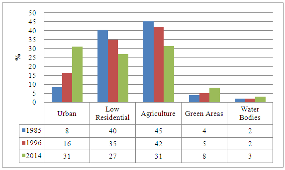Figure 3. Percentages of land uses from 1985 to 2014 in the Colombo District

The land use percentages show two important features; the urban category and the ‘green area’ category had increased, while the low residential and agriculture categories had decreased. When the percentages of land uses are compared, urban built-up shows a drastic increase of nearly 4 times from 1985 to 2014, while agricultural land had gradually decreased in the same period. The next main category of low residential also shows a steady decline over the same period, dropping to 0.325 times of the original value. Except for these three main categories, the other two land uses do not show any significant variances.

The next task s was the development of urban landscape expansion index. The above discussed different LEI (Liu et. al., 2010; Wu et al., 2010; Nong 2014) were used to develop a new landscape expansion index for Colombo district and it was named as Growth Type Index (GTI).

4.1. Growth Type Index (GTI)

Growth type index was developed to calculate landscape changes from non urban to urban. GTI was calculated using the following formula.

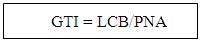GTI = Growth Type Index

LCB = Length of the Common Boundary of early and new urban patches

PNA = Perimeter of New growth Area

Growth Type Index ranges from 0 – 1 and the type of urban growth depends on the index value. Accordingly the GTI values less than 0.5 indicates infill growth and GTI greater than 0.5 indicates edge expansion growth. GTI value equal 0 indicates outlying growth. Figure 4 illustrates above different types of urban growth.

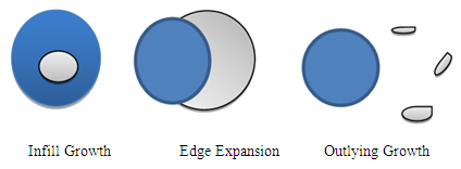Figure 4. Types of Urban Growth

Colombo District urban growth spread over in a concentric way and it varies according to the distance from the City of Colombo. Therefore, gradient analysis can be easily applied to Colombo District. Using windshield survey, most of the urban variations were identified, and these variations generally occurred at 5km intervals along main roads. Therefore, 5km buffer zones were marked on the maps of the City of Colombo until they covered the entire Colombo District, using ArcGIS 10 proximity analysis. Figure 5 shows Colombo district urban changes with distance.

Figure 5. Colombo District Land use Pattern with Distance

Within each buffer zone GTI is calculated and analysed. The results are discussed in the next section.

5. Results and Discussion

Results and discussion include types of urban growth and speed of urban growth.

5.1. Types of Urban Growth

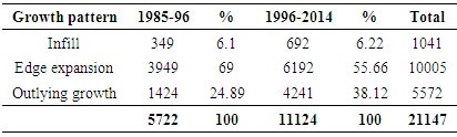
The Growth Type Index (GTI) calculated different growth types for the two different periods. Those growth types were named as infill, edge expansion, and outlying growth. After identifying the urban category mentioned in Figure 2 it was reviewed using the GTI to determine the type of urban growth; that is, whether it is infill growth, edge expansion or outlying growth. The calculated land extent in hectares coming under different growth patterns and their percentages are indicated in Table 2.

Table 2. Types of Urban Growth

Throughout the 27 year period, edge expansion was considered as the primary growth type. During the first period (1985-96) infill growth was an insignificant percentage at 6.1% while the edge expansion type accounted for 69%. Between 1996 and 2014 infill growth never showed a significant increase. However, edge expansion accounted for a considerable amount of growth but it was less than what it was in the first period. Between these two periods the outlying growth increased by 14% (from 24% in 1985-1996 to 38% in 1996-2014). Figure 5 illustrates the percentages of different urban growth during these two periods. The three urban patch growth types that were identified and the differences between their coverage at two growth periods are illustrated in Figure 6.

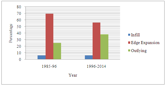Figure 6. Types of Urban Growth

As shown in the Figure 6, the main growth type at both periods was edge expansion. While it had accounted for nearly 70% of growth in the 1985-1996 period it had decreased to 55% in the 1996-2014 period. Percentage of infill growth was nearly unchanged in the two periods.

However, compared to the 1985-96 period, the outlying growth in 1996-2014 was high. There was an almost 15% increase over the 1985-96 period. Accordingly, Colombo outlying growth shows a linear and clustered growth pattern. A small percentage of isolated growth exists in few places. As the influence of the three different types of urban growth vary with the distance to the City of Colombo, it is necessary to measure the effectiveness of these growth types at different distances from the city.

5.2. Speed of Urban Growth with Distance

Firstly, the overall urban change from 1985 to 2014 in the entire district was considered; it had increased gradually from 5722 ha to 21147 ha, which correspond to 8% and 31% respectively, of the total land area Following this, the annual growth rate of urban built-up land for the two periods within the above mentioned nine buffer zones was computed. The results showed that the speed of urbanisation was different in the two study periods and tended to vary depending on the distance from the city centre (Figure 7).

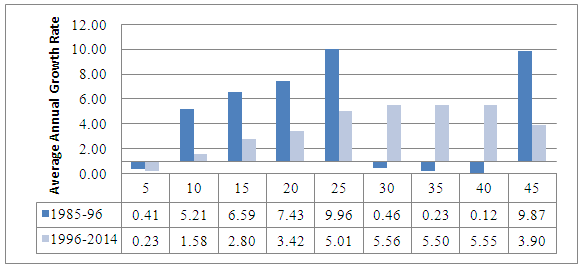Figure 7. Average Annual Growth with Buffer Distance

According to the figure, the average annual growth rate within the 5 km buffer zone did not show significant changes in both these periods and the growth rate was less than 0.5. During the period 1985-1996, the average annual growth rate within the area at 10 km to 25 km distance showed a gradual increase and the 1996-2014 growth rate also showed a similar pattern. The 1985-1996 period shows another significant feature in that the growth rate within the 30-40 km gradient was at a lower rate than 0.5. Further, the 45 km buffer zone showed a 9.87 average annual growth rate in the period 1985-96 but it decreased in the period of 1996-2014. The calculated values of the different growth types within the various buffer zones are shown in Figure 8. The growth types were considered as infilling growth, edge expansion growth and outlying growth.

According to Figure 8, more than 50% of urban growth in the 5 km buffer zone was of the infilling type but it gradually decreased as it neared the 45 km buffer zone.

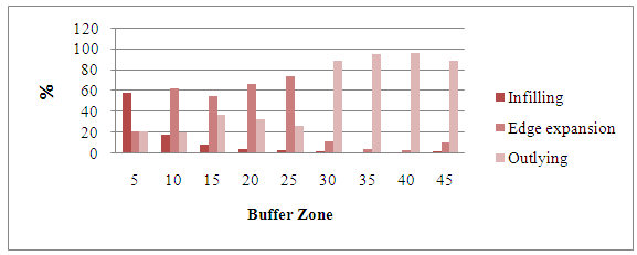Figure 8. Urban Growth in Different Buffer Zones

Edge expansion growth gradually increased as it moved from the 5 km to 25 km buffer zones. After that it decreased up to the 40 km buffer zone but showed a 10% increase in the 45 km buffer zone. Outlying growth was less than 40% from the 5 km to the 35 km buffer zone, and then it increased to more than 80% in the 30 km to 45 km buffer zones.

These changes happened mainly due to the high demand for land and the increasing land values. Residents of these areas sold their land for commercial or other urban uses, and moved to the surrounding suburban areas. The improved road and transport networks provided a further incentive to people to move to the periphery. Therefore, land use types shows urban fringe located close to the immediate suburbs of the urban core and it works as the transition region. The other part, where no significant land conversion occurred, could be considered as the outer region. Taken into consideration past urban pattern, population density move from Colombo to outer areas and urban land uses move from Colombo to outer areas. This movements help to show different variations in the different zones.

6. Conclusions

GIS integrated techniques can be used to analysed land use types and Urban Growth Index is sucessfully used for that. Further using GIS based proximity analysis those growth types were analysed with distance gradients. Colombo district land use analysis pinpointed two land use dynamics; one was that land development activities were becoming more diverse and the other was that the land development process caused fragmentation and splitting up of land. Those two patterns were further analysed using Growth Type Index for identifying urban growth types in district level. Later different types of growth were analysed using distance gradients. Accordingly, infill growth is major in first 10 km zone and up to the 25 km buffer zone the edge expansion was prominent growth type. Beyond that, up to the 40 km buffer zone, outlying growth was noticeable. It indicated that the urban fringe was gradually becoming converted to an urban area with edge expansion while the rest of the area showed outlying growth. The land use pattern presents a different picture and it shows the urban area gradually expanding by spreading out through peripheral areas with the urban fringe functioning as a transition zone.