Kiplangat Cherono Nelly , Felix Mutua
Jomo Kenyatta University of Agriculture & Technology, Department of Geomatic Engineering & Geospatial Information Systems, Kenya
Correspondence to: Kiplangat Cherono Nelly , Jomo Kenyatta University of Agriculture & Technology, Department of Geomatic Engineering & Geospatial Information Systems, Kenya.
| Email: |  |
Copyright © 2016 Scientific & Academic Publishing. All Rights Reserved.
This work is licensed under the Creative Commons Attribution International License (CC BY).
http://creativecommons.org/licenses/by/4.0/

Abstract
The quality of ground water in Juja Location is of great significance because it is the main alternative source of drinking, domestic and industrial water supply. The study aimed at mapping the potential of ground water in the Location, assess the quality of ground water and relate it to the land use and land cover. Thematic maps for the study area were generated using GIS and Remote Sensing Techniques. Reclassification and weighted overlay tools in ArcGIS software were used to generate a ground water potential map. Very low groundwater potential was observed in the northern parts of the location while high potential was observed in the central parts. Groundwater samples were randomly collected and their locations measured using a handheld GPS. The physical and chemical properties of the water were analysed in the laboratory. Spatial distribution maps of the water quality parameters were developed using Kriging method of interpolation in ArcMap software. A drinking water quality index was then developed to describe the overall quality of groundwater in the study area. Very poor water quality was observed in Mangu farm area, Gashororo area and parts of Kenyatta Road. Excellent water quality was observed in Juja farm’s Mastore area and Happy Life Children’s Home. There is an insignificant relationship between the groundwater quality and land use in the study area.
Keywords:
Groundwater quality, Geographic Information System and Remote Sensing, Spatial Distribution and Landuse/Landcover
Cite this paper: Kiplangat Cherono Nelly , Felix Mutua , Ground Water Quality Assessment Using GIS and Remote Sensing: A Case Study of Juja Location, Kenya, American Journal of Geographic Information System, Vol. 5 No. 1, 2016, pp. 12-23. doi: 10.5923/j.ajgis.20160501.02.
1. Introduction
Accessibility to water is one of the major global challenges whose impacts are largely felt in the developing countries. One of the Millennium development goals is to increase the accessibility of the population to improved sources of drinking water [1]. In Juja Location, groundwater is used as an alternative source of water supply. The occurrence of ground water is dependent on several factors including; geology, surface drainage, slope, topography, lineament density and land use/ land cover [2]. Topographic elevation and slope are important in the determination of water table elevation. The drainage pattern is important because it indicates the rate at which precipitation infiltrates into the ground. Infiltration is controlled by the permeability of the rocks which in turn is determined by the type of rocks. The amount of rainfall determines the amount and distribution of ground water because it is the source of precipitation that percolates into the ground to form ground water. In addition, some land uses allow more infiltration than others and hence affect the occurrence of ground water. Lineaments provide information on movement and storage of groundwater making it an important aspect in ground water exploration [3].Water quality is an important aspect of water resource. The quality of water is related to the source whether it is improved or unimproved. Contamination of ground water can occur due to natural or anthropogenic causes [4]. In Kenya ground water pollution has been experienced in several aquifers especially in high density informal settlements. This has been attributed to the absence of a proper sewerage infrastructure. Nitrate pollution has also been observed in Kenya particularly at livestock watering points [5]. Due to intermittency in the supply of piped water in the location and few public standpipes, the residence of Juja location have opted to supplement piped water with ground water. Boreholes are expensive to drill and therefore, the residence are left with the option of digging shallow wells to meet their water demands. Shallow unprotected wells are prone to pollution and have been associated with waterborne diseases [6]. This study focuses on assessing the quality of groundwater from shallow wells in Juja location using geospatial technologies that have proved to be very helpful.
1.1. Study Area
Figure 1 shows the map of Juja Location which is the area of interest in this study. Juja Location is located in Kiambu County, 30 km North of Nairobi City between Ruiru and Thika towns.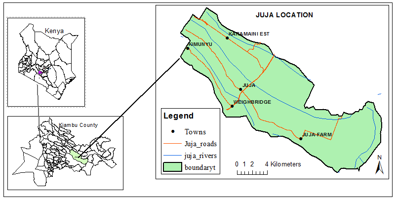 | Figure 1. Map of Juja Location |
2. Materials and Methodology
2.1. Data
The data sets that were used in the study include the Digital Elevation Model extracted from the Shuttle Radar Topography Mission (SRTM) data, Landsat 8 Operational Land Imager (OLI), the DEM and OLI were both obtained from the United States Geological Survey geodatabase, and geology data that was downloaded from International Livestock Research Institute (ILRI) geodatabase site. Figures 2 and 3 show the digital elevation model and geological characteristics of the study area respectively.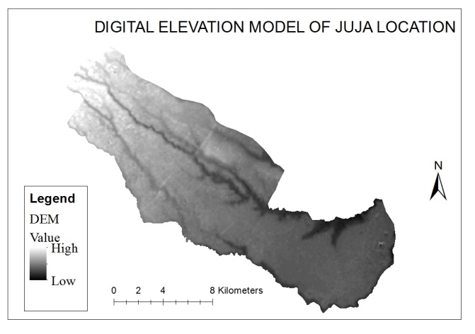 | Figure 2. Digital Elevation Model |
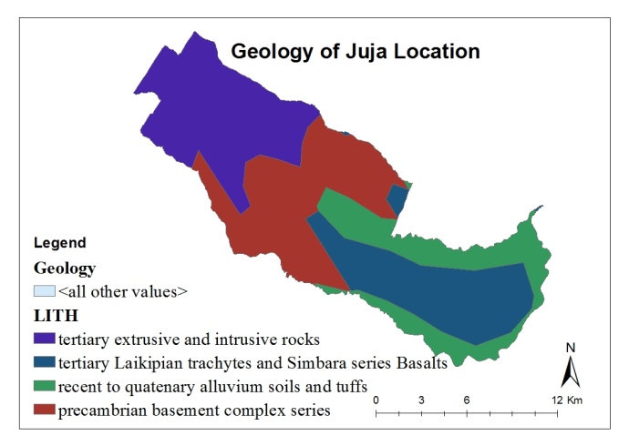 | Figure 3. Geological characteristics |
2.2. Methodology
Figure 4 shows a flowchart of the methodology that was followed during the study. The DEM was used to extract the slope, topography and flow accumulation of the study area using ArcGIS software. Lineament extraction was automatically done using the line tool in Geomatica 2014 software. The tool extracts linear features from an image and records them in a vector layer [7]. Landsat 8 image of the location was used to extract lineaments that were then exported to ArcMap software to calculate the lineament density. The land use characteristics of the study area were obtained through supervised classification of Landsat 8 image. Reclassification and weighting of the thematic layers was done based on existing literature. In order to apply the Reclassify tool in ArcMap, vector data was converted to raster format using the vector to raster tool after which all the factors were each reclassified into 5 classes, 1 being the least suitable and 5 the most suitable.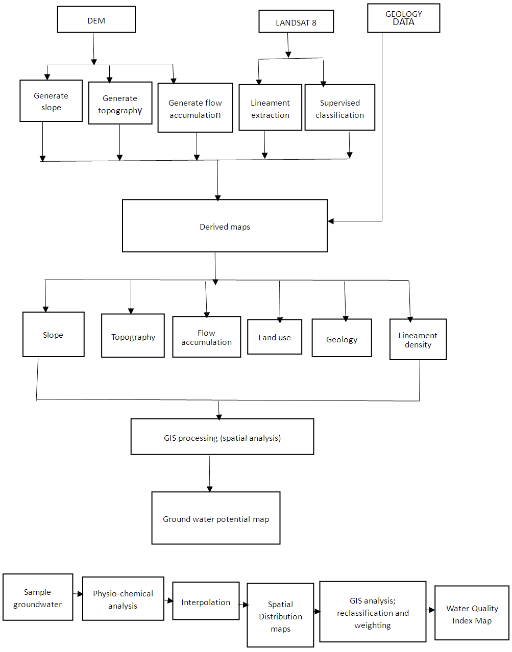 | Figure 4. Methodology Flow Chart |
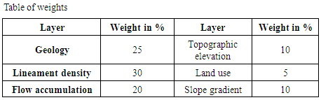
The reclassified layers were then weighted following a method modified from [8-10]. The most influential factor was assigned a high weight while the least influential factor was assigned the least weight in a scale of 0 to 100% where 0% indicates little or no influence while 100% indicated very high influence. The sum of weights should be 100%. The reclassified layers were then used as inputs in the weighted overlay tool in ArcMap 10.1 to generate a groundwater potential map. The weights assigned are shown in table 1. Table 1. Table of weights assigned to each factor
 |
| |
|
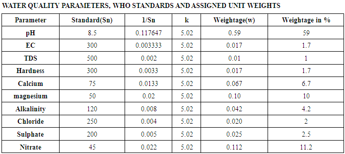
For the development of a drinking water quality index, ground water samples were collected and their locations determined using a handheld GPS. The physical and chemical properties of the water were analysed in the laboratory following standard procedures. Prediction of the water quality in the areas not sampled was done using kriging method of interpolation found in the geostatistical tool in ArcGIS software. Spatial distribution maps of various water quality parameters were then generated. The spatial distribution data of each parameter was then exported to raster using the export tool in ArcMap in order to allow for reclassification. Each parameter was then reclassified into 5 classes where 1 is the least suitable and 5 the most suitable. The WHO standards for drinking water were considered during reclassification process. Weights were calculated and assigned to each parameter according to the formula below, previously used by [11] to calculate weights. The reclassified parameters and their assigned weights were then used as inputs in the weighted overlay tool in ArcMap 10.1 software so as to generate a drinking water quality index for the study area.W = K /SnWhere W is weightage factor and Sn is the WHO standard K = [1/ (Σ ⁿ n=1 1/Sn)]Where K is the proportionality constant. Table 2 shows the water quality parameters considered in the study, WHO standards as well as their calculated weightages.Table 2. Water quality parameters, WHO standards and their calculated weights
 |
| |
|
3. Results and Discussion
3.1. Thematic Layers
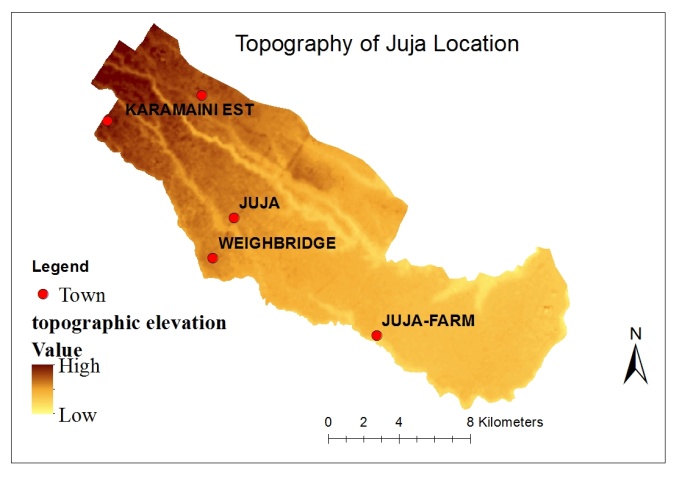
Figures 3, 5, 6, 7, 8 & 9 show the thematic layers that were used in the generation of a ground water potential map of the study area. Figure 10 shows the ground water potential map of Juja location. The ground water potential is high in the central parts of Juja location which lies under Gashororo area. This may be due to a high lineament density as well as gentle slope which encourages more infiltration of water to the ground. The ground water potential is also high along river lines due to horizontal and vertical seepage of river water into the ground [12]. There is a low ground water potential in the northern part of the location which is around Karamaine estate. This may be attributed to steep slope which encourages surface runoff and hence little percolation and infiltration [3]. The rest of the location has a moderate ground water potential.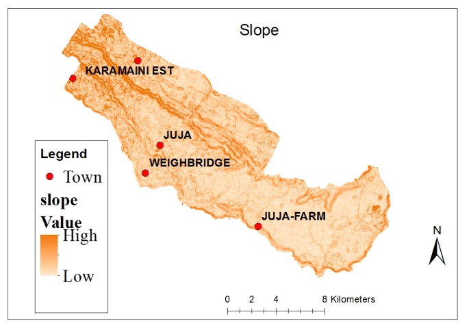 | Figure 5. Slope map |
 | Figure 6. Map of topography |
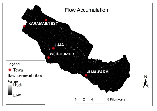 | Figure 7. Flow Accumulation Raster |
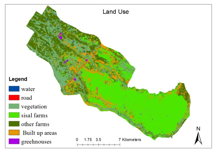 | Figure 8. Land use Map |
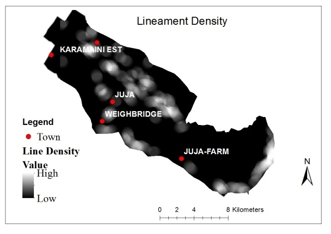 | Figure 9. Map Lineament Density |
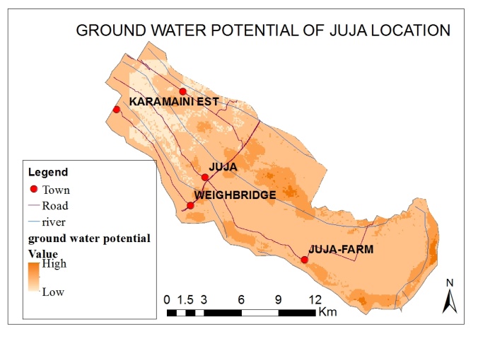 | Figure 10. Ground Water Potential Map |
3.2. Sampled Wells
Figure 11 shows the location of the randomly sampled wells in the Location. 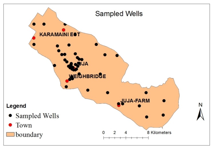 | Figure 11. Map showing the locations of sampled wells |
3.3. Spatial Distribution of Water Quality Parameters
3.3.1. pH
pH is an important property of water since it determines the suitability of water for several uses. In Juja location, the pH ranges from 5.7 to 8.9. Figure 12 shows that most areas of the study have their pH within the desirable limit of 6.5 to 8.5 which is recommended by WHO standards.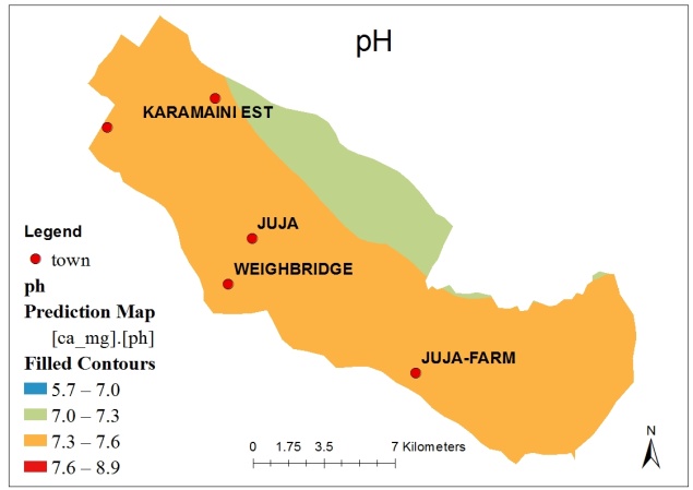 | Figure 12. Spatial distribution of pH |
3.3.2. Nitrates
High concentrations of nitrates in water cause infant methemoglobin commonly known as blue baby syndrome. The nitrate concentration in the study area ranges from 0 to 34mg/l which is within the recommended limit of 45 mg/l. High nitrate levels were recorded in the Northwest and South Western parts of the study area (figure 13).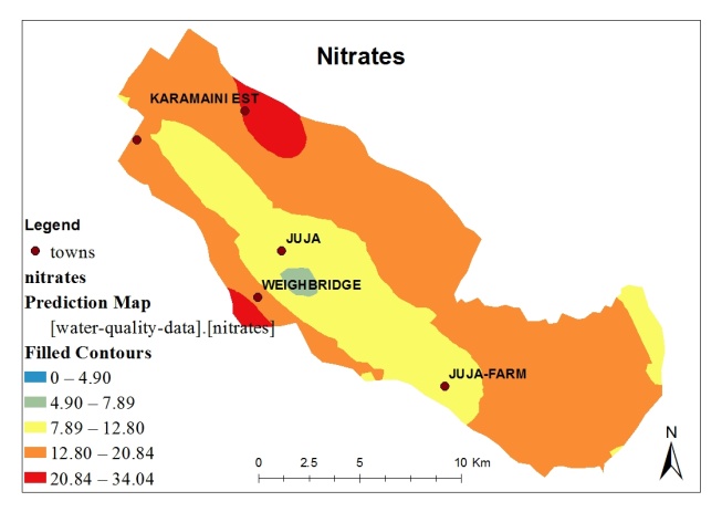 | Figure 13. Spatial distribution of nitrates |
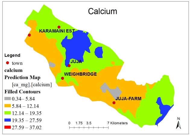
3.3.3. Calcium
Calcium is abundant in water. Both calcium and magnesium cause hardness in water. In the study area, the concentration of calcium ranges from 0.34 to 37.02mg/l which is within the recommended limit by WHO standards of 75mg/l. Figure 15 shows that high calcium levels were recorded in the northern part of the study area.
3.3.4. Alkalinity
Figure 14 shows the spatial distribution of alkalinity in Juja location. Alkalinity level ranges from 60 to 950mg/l. The desirable limit is 120mg/l. Excessive alkalinity in water causes eye irritation in human beings and chlorosis in plants. High levels of alkalinity were observed in the Southern parts of the location.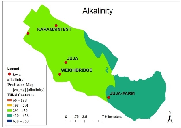 | Figure 14. Spatial distribution of alkalinity |
 | Figure 15. Spatial distribution of calcium |
3.3.5. Total Hardness
The permissible limit for total hardness in drinking water is 300mg/l of calcium carbonate. Figure 16 shows the spatial distribution of total hardness in drinking water. It ranges from 0 to 580mg/l. High concentrations were observed in the eastern parts of the study area.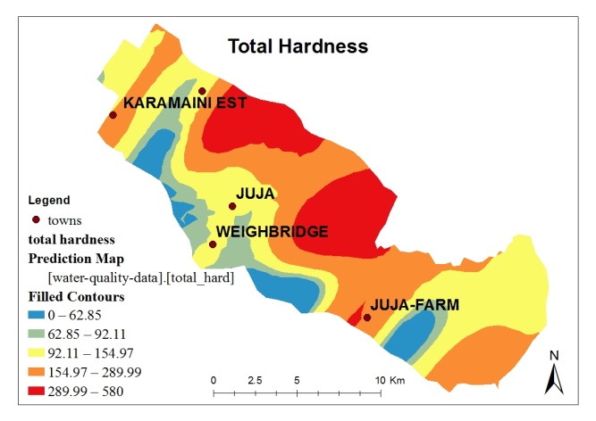 | Figure 16. Spatial distribution of hardness |
3.3.6. Chloride
Higher levels of chloride in water indicate that there is presence of organic pollutants in the water. Figure 17 shows the spatial distribution of chloride in the study area. The chloride concentration ranges from 17.8 to 345.8mg/l. The desirable limit is 250mg/l. High chloride concentrations are found in the Eastern parts of the study area while low chloride concentrations were recorded in the Central and Northern parts of the location.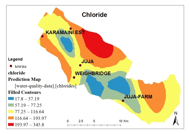 | Figure 17. Spatial distribution of Chloride |
3.3.7. Total Dissolved Solids (TDS)
According to the WHO standards, the desirable limit for TDS is 500mg/l. TDS in water is commonly caused by sewage, urban runoff and industrial wastes. Excess TDS beyond 500mg/l can cause gastro intestinal irritation. Figure 19 shows the spatial distribution of total dissolved solids in the study area. It ranges from 43 to 983mg/l. High levels were observed in the Northern parts of the study area.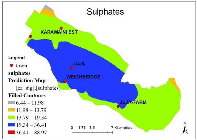 | Figure 18. Spatial distribution of Sulphates |
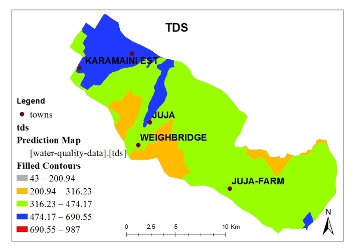 | Figure 19. Spatial distribution of TDS |
3.3.8. Sulphate
Sulphates can naturally occur in water due to soil and rock formations. As water passes through the soil and the rocks, sulphates are picked and they get dissolved in ground water. Figure 18 shows the spatial distribution of sulphates in ground water of the study area. The concentrations vary from 6.44 to 88mg/l. The permissible limit is 200mg/l.
3.3.9. Magnesium
Magnesium concentrations in the study area range from 0.28 to 2.5 mg/l. The maximum allowable limit for magnesium according to the WHO standards is 50mg/l. Magnesium causes water hardness. Figure 21 shows the spatial distribution of magnesium in the study area. High magnesium concentrations were observed in the eastern parts of the study area.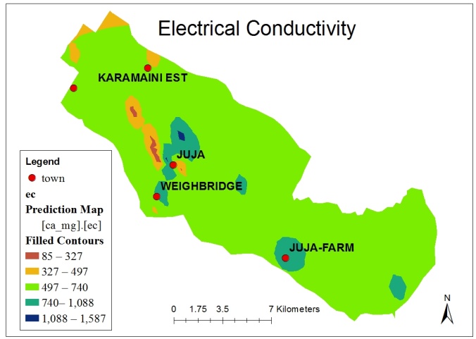 | Figure 20. Spatial distribution of EC |
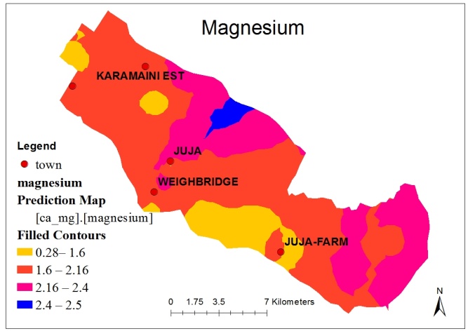 | Figure 21. Spatial distribution of Magnesium |
3.3.10. Electrical Conductivity
Electrical conductivity is the ability of electrical current to pass through water. Figure 20 shows the spatial distribution of electrical conductivity in the study area ranging from 85 to 1587. The permissible limit is 300 micro Siemens. EC is associated with excessive water hardness.
3.4. Water Quality Index
Figure 22 shows the drinking water quality index of the study area. Generally, most areas of the location have good water quality which is fit for drinking. However, the water quality is poor in Mangu farm, Gashororo, sewage and Umoja estate. In Mangu farm, this may be due to mismanagement of the coffee farms including improper management of fertilizers, pesticides, herbicides and insecticides. In Gashororo, Sewage and Umoja areas, the poor water quality may be due to poor solid and liquid waste management. The major solid waste disposal means is open dumping. Poor sewerage infrastructure may be another cause of ground water contamination. The residents of the area use open sewage to dispose their liquid wastes. The septic tanks are also poorly designed. The water in this areas is high in electrical conductivity, TDS, and alkalinity exceeding the recommended WHO standards. The water is also acidic indicated by low pH values. The area around Mastore and happy life children’s home has excellent groundwater quality which may be attributed to sisal farming whose production does not involve the use of inorganic fertilizers. This limits chances of groundwater contamination.  | Figure 22. Water Quality Index Map |
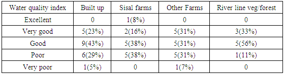
Table 3 shows statistics of sampled wells, land use and water quality. Of all the wells that were sampled in built up areas, 23% were found to have very good water quality, 43% were of good quality while 34% had poor and very poor water quality. In sisal farms 8% had excellent water quality, 16% and 38% had good and very good water quality respectively while 38% had poor water quality. Of the wells that were sampled in other farms including coffee farms, maize farms among others, 62% had good water quality and 7% had poor water quality. The wells that were sampled in forested areas, 89% had good water quality while 11% had poor water quality. Low R2 values (figure 23), obtained from the geographically weighted regression model indicate an insignificant relationship [13]. The poor water quality may be due to mismanagement practices.Table 3. Water quality statistics
 |
| |
|
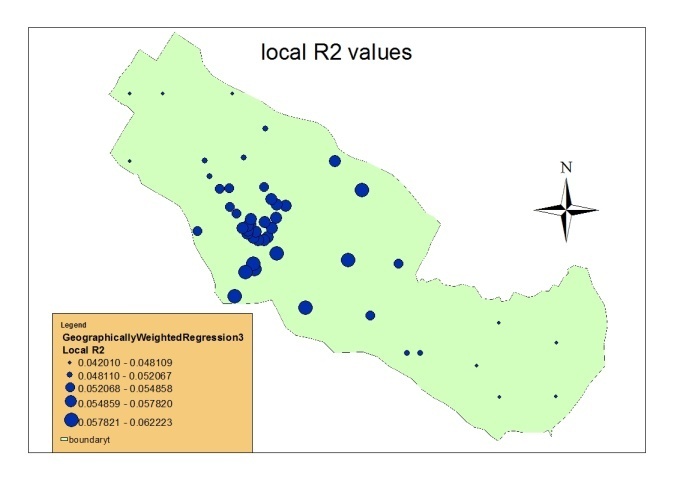 | Figure 23. Map showing local  values values |
4. Conclusions
The ground water potential of Juja location was explored through carrying out weighted overlay of thematic maps including; geology, lineament density, land use, surface drainage, slope and topography. The Northern parts of the location have the lowest ground water potential. This are areas around Karamaine Estate. The central parts of the location which lies under Gashororo area and the areas along rivers have a high groundwater potential. Most parts of the location have moderate ground water potential which can be exploited to meet water demands.The drinking water quality index that was generated for the study area shows that the eastern parts of the location specifically Mangu farm has the poorest water quality. The central parts around Gashororo and sewage areas also have poor drinking water quality. In Juja farm area around Mastore and Happy life Children’s home, the ground water is of excellent quality. The rest of the location has good drinking water quality. There is no significant relationship between land use and ground water quality in the study area. The poor water quality in the mentioned areas may be attributed to mismanagement practices like poor waste management and poor farm management practices.
AKNOWLEDGEMENTS
I would like to acknowledge my supervisor Dr. Felix Mutua for his guidance throughout the research period. I also would like to thank the Jomo Kenyatta University GIS lab technicians; Mr. Muruiki, Mr. Waswa and Ms. Sarah for their technical support in the research. Finally I would like to thank my husband Nicholas, my son Brandon and my parents for their financial and moral support throughout the research period.
References
| [1] | United Nations. (2013). Millennium Development Goals Report |
| [2] | Ndatuwong, L. G., & Yadav, G. S. (2014). Integration of hydrogeological factors for identification of groundwater potential zones using remote sensing and GIS techniques. Journal of Geosciences and Geomatics, 2(1), 11-16. |
| [3] | Rahmati, O., Samani, A. N., Mahdavi, M., Pourghasemi, H. R., & Zeinivand, H. (2015). Groundwater potential mapping at Kurdistan region of Iran using analytic hierarchy process and GIS. Arabian Journal of Geosciences, 8(9), 7059-7071. |
| [4] | Watkins, K. (2006). Human Development Report 2006-Beyond scarcity: Power, poverty and the global water crisis. UNDP Human Development Reports (2006). |
| [5] | Muma A., Lane I.M., & Kairu E.N. (2010). Kenya Groundwater Governance Case Study. |
| [6] | Mwaniki M., Waithaka E., Ngigi T & Gachari. (2011). Determination of Safe Distances between Shallow-Wells and Soak pits within Plots in Juja, Kenya. |
| [7] | PCI Geomatica 2014. (n.d.). Geomatica Help. |
| [8] | Umikaltuma Ibrahim Mohamed. (2014). Investigating the Groundwater Potential of Gedo Region, Somalia, Using Geospatial Technologies. |
| [9] | Musa KA, Juhari Mat A, Abdullah I. (2000) Groundwater prediction potential zone in Langat Basin using the integration of remote sensing and GIS. The 21st Asian Conference on Remote Sensing, Taipei (Taiwan). |
| [10] | Sener, E., Davraz, A., & Ozcelik, M. (2005). An integration of GIS and remote sensing in groundwater investigations: a case study in Burdur, Turkey. Hydrogeology Journal, 13(5-6), 826-834. |
| [11] | Asadi, S. S., Vuppala, P., & Reddy, M. A. (2007). Remote sensing and GIS techniques for evaluation of groundwater quality in Municipal Corporation of Hyderabad (Zone-V), India. International journal of environmental research and public health, 4(1), 45-52. |
| [12] | Gupta, M., & Srivastava, P. K. (2010). Integrating GIS and remote sensing for identification of groundwater potential zones in the hilly terrain of Pavagarh, Gujarat, India. Water International, 35(2), 233-245. |
| [13] | Tu, J., & Xia, Z. G. (2008). Examining spatially varying relationships between land use and water quality using geographically weighted regression I: model design and evaluation. Science of the total environment, 407(1), 358-378. |

 Abstract
 Reference
 Full-Text PDF
 Full-text HTML