Peter M. Macharia 1, Charles N. Mundia 2, Miriam W. Wathuo 1
1School of Pure and Applied Sciences, Pwani University, Kilifi, Kenya
2Institute of Geomatics, GIS and Remote Sensing, Dedan Kimathi University of Technology, Nyeri, Kenya
Correspondence to: Peter M. Macharia , School of Pure and Applied Sciences, Pwani University, Kilifi, Kenya.
| Email: |  |
Copyright © 2015 Scientific & Academic Publishing. All Rights Reserved.
This work is licensed under the Creative Commons Attribution International License (CC BY).
http://creativecommons.org/licenses/by/4.0/

Abstract
Analytical Hierarchical Process (AHP) relies on expert responses to capture a decision maker's point of view on different application domains, which is fundamental to the credibility and quality of decisions made. Do we know what experts/respondents take into consideration when they give responses? How does their knowledge influence the responses they give? It seems obvious that opinions should be sought from experts in diverse fields in a Geographical Information Systems (GIS) based oil pipeline routing using AHP. Is this an assumption that should be made? Do experts in the same area of expertise make decisions based on their professional knowledge or do they make subjective judgment irrespective of their profession? Their decisions, whether rational or subjective, will have an input on the final proposed pipeline route. This study compared the weights of 13 variables to be considered in pipeline routing derived using AHP in a GIS based pipeline routing process from the responses of six groups comprising of civil engineers, environmentalists, county administrators, local residents of the study area, oil industry experts, and geoinformation experts. Comparison of the responses was done among experts of the same group and between groups using the Spearman's rank correlation coefficient. Intraclass Correlation Coefficients (ICCs) were used to measure the reliability or consistency of rating the different variables by the experts. Visual comparison of the responses was done using scatter plots and bar graphs. Out of the six groups of experts, geoinformation specialists gave closely related responses and county administrators gave moderate related responses amongst themselves, while the rest gave relatively varied responses. It was shown that most individuals made subjective decisions, due to the large variation of responses within groups of similar profession. There was little correlation within the groups of oil experts, environmentalists and local residents. The consistency of rating of different variables by these groups was also low. In these groups, there was lower reliability level if we were to seek responses from only one expert in each of the groups. From the analysis between groups, consistency of rating of the variables by the different groups was high, but the reliability if we were to ask one group was low. Therefore, it was concluded that responses should be sought from different groups of experts, having the expertise required in pipeline routing, with each group having several respondents. However, experts should respond based on their professional knowledge. Else, the need to seek responses from different experts in a group, and from different professional groups loses its meaning.
Keywords:
AHP, Experts response, GIS, Pipeline routing, Statistical Analysis, Variation
Cite this paper: Peter M. Macharia , Charles N. Mundia , Miriam W. Wathuo , Experts’ Responses Comparison in a GIS-AHP Oil Pipeline Route Optimization: A Statistical Approach, American Journal of Geographic Information System, Vol. 4 No. 2, 2015, pp. 53-63. doi: 10.5923/j.ajgis.20150402.01.
1. Introduction
There are various variables considered in a pipeline routing process. Therefore it is necessary to rank each variable in order of importance. This helps determine the influence each variable has on the routing process. The GIS approach to pipeline routing optimization is based on relative rankings and weights assigned to project specific factors that may affect the potential route. This results in an optimal path which maps out the most economic path between the start and end points of the pipeline [1]. The factors influencing pipeline route selection are technical and engineering requirements, environmental considerations, and population density [2].AHP is a multi-criteria decision making method originally developed in 1980. It is a quantitative method for decision ranking which involves developing a numerical score to rank each decision alternative based on how well each alternative meets the decision maker’s criteria [3]. The process aids in the solution of complex multiple criteria problems in a number of application domains, such as making decision alternatives and weighting factors affecting an application.In AHP, one constructs hierarchies then performs measurements on pairs of elements with respect to a control element to obtain ratio scales, which are then incorporated into the whole structure to select the best alternative. The ratio scales are derived from the principal Eigen vectors and the consistency index is derived from the Principal Eigen value [4]. This study analyses the results of weights derived from expert responses on an oil pipeline routing using AHP and GIS. The routing process and results have been described elsewhere [5].
1.1. AHP and GIS in Practical Use
GIS and AHP have been used together in many applications. In previous studies, GIS has been used primarily for spatial analysis while AHP has been used for either evaluating different alternatives or weighting different factors to come up with a new solution. In the GIS domain, AHP has been applied in two distinctive ways. Firstly, it has been used to derive weights associated with attribute map layers. The weights are then combined with the attribute map layers. This is applicable when it is impossible to perform a pairwise comparison of the alternatives [6]. This method is popular because it is very easy to implement within the GIS environment, easy to understand, and intuitively appealing to decision-makers [7]. Secondly, AHP has been used to aggregate the priority for all levels of the hierarchy structure including the level representing alternatives. Thus, a relatively small number of alternatives can be evaluated [8].Suresh et al integrated GIS and AHP in coming up with an optimal pipeline route in India. GIS was used for analysis while AHP was used for weighting. A questionnaire was used to perform pairwise comparisons so that an expert could quantitatively rank one criteria over another to come up with weights. A sub questionnaire was also designed to counter the effect of variation in the different classes of a single criteria in routing a pipeline. Three experts were presented with the questionnaires and their weights averaged. Two routes were developed, one with AHP weights and another without. Results showed that the route generated using AHP based weights scored over the latter [9].Jianhua et al, used AHP and GIS to come up with a pipeline route. GIS was used for spatial analysis modelling and data overlay, while AHP was used to rank different factors affecting a pipeline route. This aided in reducing the impact of subjective factors, thus the generated pipeline route was more reasonable and effective. They concluded that the introduction of AHP into GIS-based oil and gas pipeline route selection system aids in weighting influential factors. Therefore, AHP method could make oil and gas pipeline route selection more effective [10].Bunruamkaew conducted a study in Thailand to identify and prioritize the potential ecotourism sites in Surat Thani province, using GIS and AHP. GIS provided a mechanism for spatial analysis while AHP was used to weight the different factors that affect an eco-tourism site location. This was done by use of questionnaires provided to 30 experts, with only 21 being consistent [11].A research which was done by Alex et al to conduct a risk assessment of pipelines, incorporated AHP. They achieved this objective by determining the relative contribution of different failure factors to the overall pipeline failure. Six pipeline experts were provided with AHP based questionnaires [12]. In determining a least‐cost path for optimal haulage routing of dump trucks in large scale open‐pit mines multiple AHP and GIS was used. The weights of five factors was derived using pairwise comparisons [13].In order to explore the use of AHP in selecting an appropriate irrigation method, a study was carried out in four provinces in Iran. A panel of experts utilized AHP to determine the priority of three irrigation methods for four group of farmers [14].
1.2. AHP Inconsistencies Studies
Nevertheless, many research are continually being done to understand the inconsistencies that arise when AHP method is used.A method was proposed for quantitative estimation of the decision maker's knowledge in the context of AHP in cases where the judgment matrix is inconsistent [4]. Dong et al derived two consensus indexes for AHP to help decision makers reach a consensus and provide more convincing alternatives. These are the geometric cardinal consensus index, and the geometric ordinal consensus index, to measure the consensus degree among judgment matrices or decision makers [15]. Lin et al, introduced uncertainty theory to deal with non-deterministic factors in ranking alternatives. The uncertain variable method and the definition of consistency for uncertainty comparison matrices were proposed. An approach for testing whether or not an uncertainty comparison matrix is consistent was put forward. AHP was examined to illustrate the validity and practicality of the proposed methods [16]. More research is continually being carried out to understand any inconsistency in the AHP method. Very few, if any, studies have been carried out to understand the variation of experts’ responses in professionally homogeneous groups and the rationale of such groups. This research aims to understand the variation of experts’ responses in a group and between groups, to enable us decide if we should seek the opinion of just one expert irrespective of profession, several experts from different professional groups, or just one expert for each relevant professional group, to help in coming up with an optimal pipeline route.
2. Methodology
2.1. Study Area and Datasets
The study area extended between 0°51N and 1°7’S and approximately between 38°36 E and 35°18’E. It bounded the counties of: Laikipia, Nyeri, Nyandarua, Meru, Nakuru and parts of Isiolo in Kenya as shown in Figure 1a below. 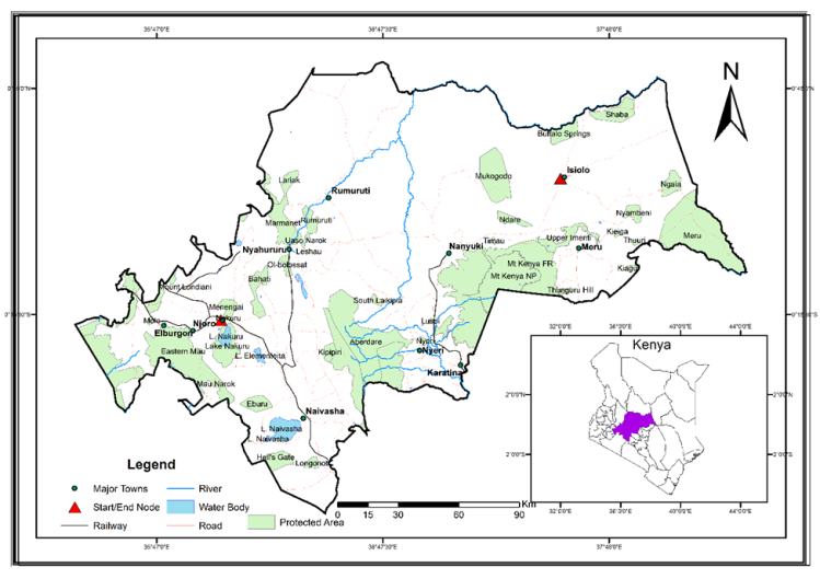 | Figure 1a. Study area |
The primary dataset used was the weights derived from experts’ responses using the AHP method. The process of coming up with a route for a pipeline has been described elsewhere by Macharia et al [5]. The different groups of experts were chosen to have a holistic representation of professionals used in an oil pipeline routing process.
2.2. Participants Selection
We approached 50 individuals, out of which 40 agreed to participate in the study. The main reason given by those who did not wish to participate in the study was that filling the questionnaires needed a lot of time and a high level of concentration. Questionnaires from 8 respondents were declared invalid because they were not filled according to instructions. Experts who participated in the study included civil engineers, environmentalists, geoinformation experts, oil and pipeline industry experts, county administrators, and residents living in the potential area where the pipeline would pass. They were recruited from the government, private entities, institutions of higher learning, and the local community.Environmentalists were recruited from the National Environmental Management Authority (NEMA), a government parastatal while civil engineers were recruited from the Jomo Kenyatta University of Agriculture and Technology (JKUAT) department of civil and environmental engineering and private practice. Geoinformation experts (GIS and remote sensing experts, surveyors, and geomatic engineers), were recruited from JKUAT's department of Geomatic Engineering and GIS, and from the Kenya Power and Lighting Company. County administrators were government officials in Nairobi County, formerly chiefs, district officers, and district commissioners. Oil and pipeline experts were sought from employees in private oil companies. The experts were approached in their respective places of work to avoid inconvenience and encourage participation as there was no compensation provided to respondents. The process of answering the questionnaires was explained briefly in the questionnaire itself and verbally. The experts either agreed or declined to be part of the study. This exercise was conducted from April to November 2013.
2.3. AHP Weighting
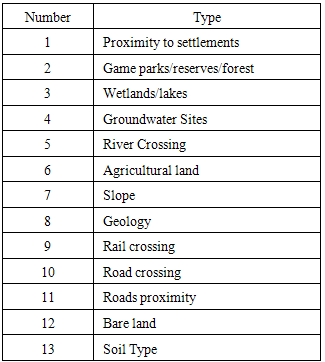
Using the variables applicable in routing a pipeline in a typical Kenyan landscape as shown in table 1, we used AHP to calculate weights from the ranks given by the experts.Table 1. Variables used in the Study
 |
| |
|
Experts were presented with a questionnaire (Figure 1c) with the 13 variables each to be compared against all the other. This resulted into 78 pairwise comparisons. The expert responded to a pairwise comparison, by indicating the relative importance of the two variables on a scale that has been proposed by Thomas L Saaty [17].The experts compared two factors at a time, e.g. road crossing versus proximity to settlements. If an expert ticked, say 7, on the side with proximity to settlements, this meant that settlements were 7 times more important than a road crossing. Therefore, it was more preferable if the pipeline crossed a road rather than passing near settlements. If the expert ticked 1, then he/she did not feel that either variable was superior to the other. The methodology used to derive weights is depicted in the Figure 1b below. 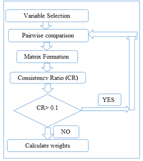 | Figure 1b. Flow chart for AHP weighting |
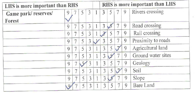 | Figure 1c. An Extract of answered questionnaire |
Variable selection was done at data collection point. Thirteen variables were selected [5] and used to form the pairwise comparisons. The rationale for selection of each variable was explained to the respondents e.g. routing near/along roads for accessibility and utilization of existing linear disturbances.While it’s common for variables to be grouped into broader categories, this study didn’t group the variables. This method of deriving weights associated with attribute map layers is of particular importance for problems involving a large number of alternatives, when it is impossible to perform a pairwise comparison of the alternatives [6]. Further this approach was used to make sure that any effect a variable has, however small, was accounted for. Roads, for example, has two categories. The first is road crossing, which caters for the fact that one may want to avoid a scenario where a pipeline crosses the road to reduce construction cost and traffic jams. The second is roads proximity, which caters for the idea of routing along the road to reduce creation of more linear disturbances while utilizing the existing ones. Further, some factors such as rivers and lakes could be grouped together as environmental factors, but there could be a scenario in which an expert would opt to allow a river to be crossed instead of a lake due to cost and level of environmental impact. Due to this, variables were not grouped.A matrix for each respondent was formed in order to calculate the weights and the consistency ratio. If the consistency ratio (CR) was acceptable weights were calculated. Otherwise, the pairwise comparison was redone. The process was repeated twice, and if the CR was still found to be unacceptable, the respondent was considered inconsistent. Results of the inconsistent respondents were not included in the analysis.
2.4. Statistical Analysis
These results were further analyzed statistically to detect the similarities and variations in each group of experts and among the groups in order to assess the need to seek opinions from experts of different fields.Statistical analysis was done using STATA version 13.1 (StataCorp US). The dataset columns consisted of the ratings of each expert on each variable, while the rows had ratings for one variable by each expert. Spearman's correlation coefficient, scatter plots and bar graphs were used to analyse the relationship between responses of experts within the same group and between different groups. The confidence level assumed was 95%, but a Šídák adjustment was applied to minimize the chances of making a type I error. A Šídák adjusted p-value less than 0.05 meant rejecting the null hypothesis that responses were uncorrelated.A correlation of 0 meant no correlation between the responses. 0.30–0.49 was interpreted as a weak correlation between responses, while 0.50–0.69 was considered a moderate correlation. Correlations above 0.70 were considered as a very strong relationship between the experts’ responses, while 1 meant perfect correlation between the responses. A negative correlation is a sign of an inverse relationship between two variables. In this study, a negative correlation between the responses of two experts meant that for most of the variables that one expert rated highly, the other one gave them a low rating. Thus, negative correlations were interpreted as total disagreement between two respondents. We also sought to establish if the various groups of experts were consistent with each other in the way they provided their responses. The dataset was transformed to long format, which was necessary for the calculation of Intraclass Correlation Coefficients (ICC) using STATA. The ICCs were used to measure the reliability or consistency of ratings of the different variables by the experts. We used the two-way random-effects ICCs to estimate the consistency of agreement of the ratings among the considered experts. This generated two measures, one of which was the average measures ICC, a measure of the consistency of agreement among raters, also known as Cronbach’s alpha. The second measure was the individual measures ICC, which gave an estimate of how reliable the responses would be if we were to only consult one expert.A 95% confidence level was also assumed and p-values less than 0.05 were taken to mean that there was evidence of some level of consistency between the responses of the experts. However, any negative ICC measures were reported as 0.00 because negative consistency does not make sense theoretically.Values for both average and individual measures were interpreted like those of Spearman's correlation coefficient.
3. Results and Discussion
The results are presented in terms of each group of experts and comparison between the groups. The order in which the variables are listed in Table 1 is the same order in which they appear on the horizontal axis of the bar graphs.
3.1. Geoinformation Experts
The resultant weights showed that wetlands/lakes and groundwater sites were some of the most highly rated variables, while road crossing and bare land were some of the variables that these experts gave low rating. Figure 2 below shows the variation of the ratings from these experts.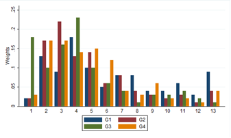 | Figure 2. Geoinformation (G) weights |
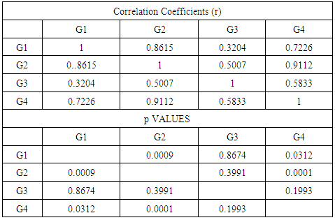
According to correlation coefficients generated and shown in Table 2 below, experts 2 and 4 had the highest level of agreement, with a correlation of 0.91, which was highly significant (p = 0.001). Agreeability among experts 1, 2 and 4 was good, and the correlations were statistically significant. However, the relationships between expert 3 and all other experts was not statistically significant, showing that all experts in this group seemed to agree in their responses, apart from expert 3. The scatter matrix shown in figure 3 below supports the above statements, as most of the scatter plots show a positive linear correlation. The scatter matrix shown in figure 3 below supports the above statements, as most of the scatter plots show a positive linear correlation. 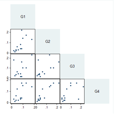 | Figure 3. Scatter Matrix of Geoinformation (G) experts |
Table 2. Geoinformation Experts p and r values
 |
| |
|
From the ICC, the consistency of the experts in rating the various variables was 0.87 (95% CI 0.70 – 0.96), which shows a strong level of consistency. The reliability level of using a single engineer to rate these variables was 0.63 (95% CI 0.37–0.85), which was good. The reliability levels were statistically significant (p<0.001). In the scatter matrix in figure 3 below, relationships between each expert and all the experts in the geoinformation group is shown. G1 versus G2 (Geoinformation expert 1 versus Geoinformation expert 2) is shown by the intersection of G1 and G2. The intersection of a column and a row shows the relationship of the corresponding two experts. This applies to all the scatter matrices in this article.
3.2. Civil Engineers
The civil engineers consulted were those mainly involved in linear routing especially for pipelines and highways. Proximity to settlements and game park/reserves/forests were rated highly by most of the civil engineers. On the other hand soil type and bare land variables were given a low rating. In this group, engineer one's responses were observed to have the greatest variation from those of the other engineers. Figure 4 shows the variation in terms of weights by the engineers.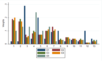 | Figure 4. Variation of civil engineers (E) weights |
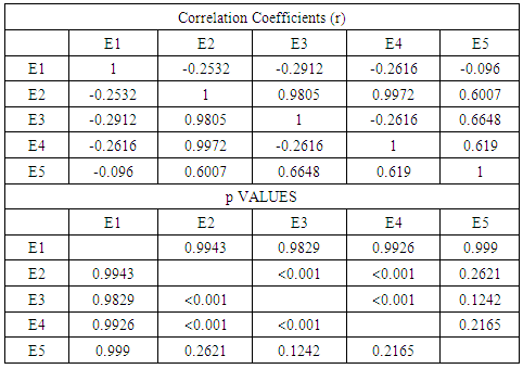
There was strong correlation between responses of engineers 2, 3 and 4. For example, the correlation between engineers 2 and 4 was 0.997, which was highly significant (p<0.001). Engineer 1 and 5, on the other hand, did not seem to agree with the other engineers because the relationships between engineers 1 and 5 and other engineers were not significant, meaning that there is no evidence that the responses were correlated. Table 3 below shows p values and correlation coefficients(r). The scatter matrix in figure 5 below shows an almost perfect linear relationship between the responses of some experts (engineer 2, 3 and 4), while for some experts (engineer 1 and 5), there is no observable pattern in the scatter plots.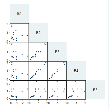 | Figure 5. Scatter matrix of Civil Engineers |
Table 3. Civil Engineers’ p and r values
 |
| |
|
The consistency of the experts in rating the different variables was 0.68 (95% CI 0.29 – 0.89), which was good. However, the level of reliability if we were to get responses from only one engineer was 0.30 (95% CI 0.08 – 0.62), which was quite low. These values were statistically significant (p=0.002). In this category, it is evident that only 3 individuals had highly correlated responses, thus there was some level of bias applied.
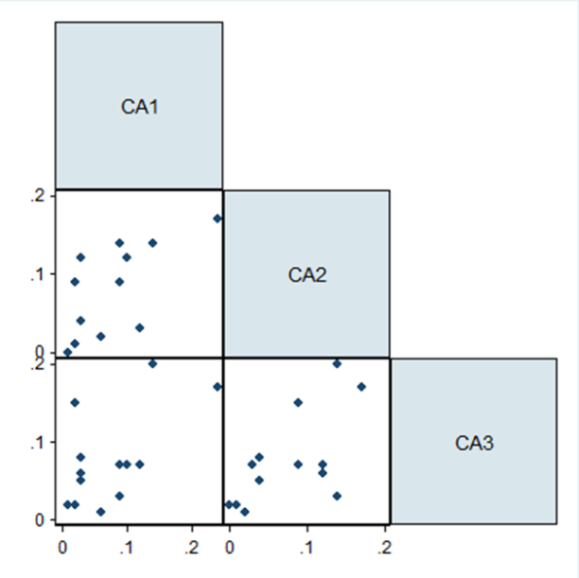
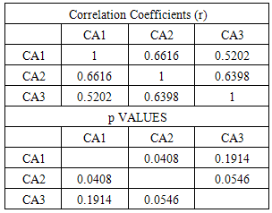
3.3. County Administrators
Individuals who fell into this category were former chiefs, district commissioners and district officers. Some of the variables that were rated highly by most county administrators are proximity to settlements and agricultural land, while geology and bare land were rated lowest. The correlations in table 4 show moderate correlation between the responses of all three county administrators, however, only the relationship between the responses of experts 1 and 2 was statistically significant (p=0.04). This shows a moderate level of agreement among these individuals. Figure 6 below shows the variations of ratings. There was good consistency of rating among the individuals as the average measures ICC value was 0.83 (95% CI 0.56 – 0.94). The level of reliability if we were to get responses from only one county administrator was 0.62 (95% CI 0.30 – 0.85), which is a good level. The reliability measures were statistically significant (p<0.001). 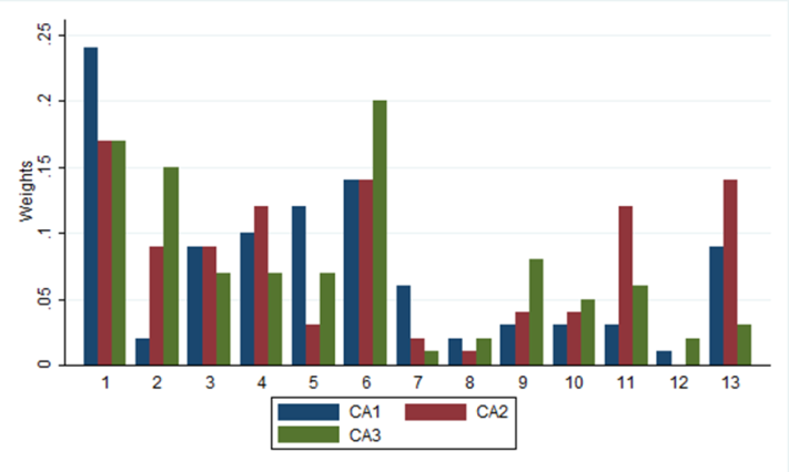 | Figure 6. Weights variation by County Administrators |
 | Figure 7. Scatter matrix for county administrators |
Table 4. County Administrators’ p and r values
 |
| |
|
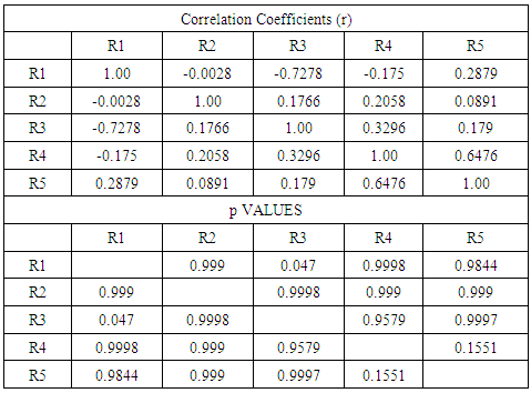
3.4. Local People/Residents
This category included people who were residents of the study area, but did not have a specific area of expertise. There was no specific preference for a certain variable in this category, and no relationship between the residents’ responses was statistically significant as shown in table 5 exception of resident 1 and respondent 3. This shows total disagreement between the residents. Most of the scatter plots in the scatter matrix show no pattern, suggesting very low level, if any, of agreeability among the residents. This can be attributed to the fact that while a person may be a resident of a particular county, their point of view might not be that of a county resident. Figure 8 shows this variation.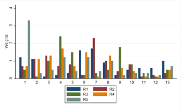 | Figure 8. Variation of Locals response |
Table 5. Local people/ Residents’ p and r values
 |
| |
|
This is further supported by the reliability values from the ICC. The consistency of rating among the residents was quite low, at 0.16 (95% CI 0.00 – 0.71), while the reliability level if we had sought responses from only one resident was at 0.04 (95% CI 0.00 – 0.33). However, the reliability measures were not statistically significant. This means that there is not enough evidence to conclude that there is consistency among the residents. The scatter matrix in Figure 9 shows that the variables have no relationship. 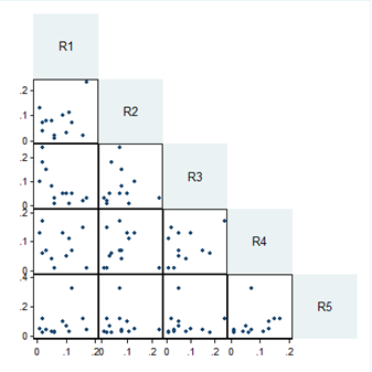 | Figure 9. Scatter matrix for residents |
3.5. Environmentalists
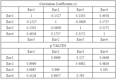
Wetlands/lakes and groundwater sites were rated highly by most environmental experts. Game parks were also given importance by most experts in this category while bare land and rail crossing received low ratings, according to figure 10. In this category, there was no relationship between responses that was statistically significant as shown in table 6. This means that there was not enough evidence to conclude that the responses between any of the environmental experts were correlated. Generally, all environmentalists differed in their responses. 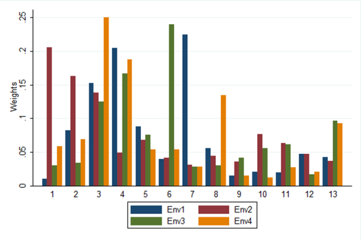 | Figure 10. Variation of weights by Environmentalist |
Table 6. Environmentalists’ p and r values
 |
| |
|
The consistency of rating among the environmental experts was weak, at 0.48 (95% CI 0.00 – 0.82), and it was not statistically significant (p=0.07). There was no evidence to conclude that there was any consistency of rating among the environmentalists. If we were to ask only one environmentalist, the reliability would be 0.19, which is quite low. The scatter matrix in Figure 11 below shows the variations between the responses. 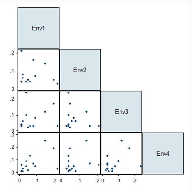 | Figure 11. Scatter matrix for Environmentalist |
3.6. Oil and Pipeline Experts
Only two experts’ responses were considered for this category and they had very different opinions as shown in figure 12. The relationship between the responses of the two experts was not statistically significant (p=0.39), which shows that their responses were completely different, as there was no evidence to support that there was any relationship between their responses.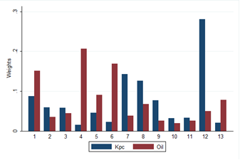 | Figure 12. Weights variation by Oil/Pipeline experts |
The scatter plot also shows no pattern in the data. The calculated consistency of agreement between the experts' was not statistically significant (p=0.83), implying that there was not enough evidence to conclude that there was any consistency between the ratings of the two experts. 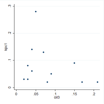 | Figure 13. Scatter plot for oil experts |
3.7. Group Analysis
A comparison of the various categories of the group of experts is shown by Figure 14. Various factors were rated similarly based on the percentages calculated. Road crossings and proximity and rail crossings all averaged to least rated. For bare land, only the oil experts differed with the rest. Ground water sites, slope, game parks and agricultural land had majority of experts giving similar percentages. Settlements, geology and wetlands were seen to have varying percentages. 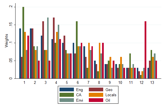 | Figure 14. A comparison of various categories of weights |
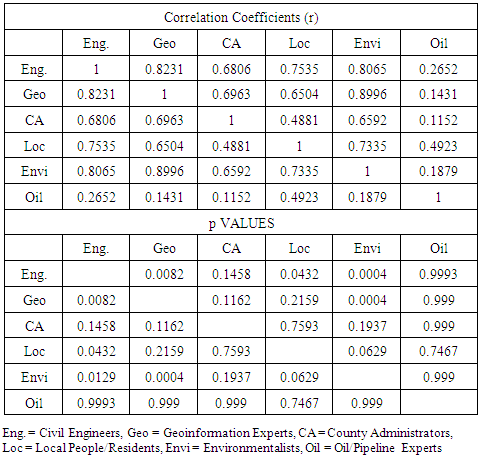
We compared the responses of all the experts, using average responses from all groups, to see which groups of experts agreed more or disagreed in their opinions. From table 7 of correlations, geoinformation experts and environmetalists had the highest correlation in their responses, at 0.8996 (p=0.0004), which suggests that their level of agreement was high. Geoinformation experts and engineers also had a high level of agreement, with a correlation coefficient of 0.8231 (p=0.0082). Oil experts and county administrators had a completely different opinion from other experts, while the engineers seemed to have a high level of agreeability with all the other experts apart from oil and pipeline experts and county administrators. Out of 15 comparisons only 4 had high correlations that were statistically significant. Therefore it can be shown that the groups did not relate to each other.Table 7. Groups of experts p and r values
 |
| |
|
The average measure value among the different experts was 0.81 (95% CI 0.59 – 0.93), which was quite high, and the consistency was statistically significant (p<0.001). However, the level of reliability if we were to consult only one group was low (0.42), and despite the high value of Cronbach's alpha, we conclude that the consistency of agreement between groups was low.
4. Conclusions
The responses given by experts in a pipeline routing process using GIS and AHP are used to influence decisions made by policy makers. Therefore, the nature of the responses contributes directly to the credibility and the quality of the decision made. Geoinformation experts gave closely related responses amongst themselves with exception of one expert while county administrators gave moderate related responses. Three out five civil engineers agreed amongst themselves. On the other hand, oil and pipeline experts, environmentalists, and residents of the study area had varied responses amongst themselves. Furthermore, only geoinformation experts and county administrators had a high individual measures figure, meaning that we could have relied on one expert from each of these groups to give us reliable responses. This shows that it is necessary to seek the opinion of different individuals from the same profession or group. The analysis of the averages of the groups showed that there was little correlation between most groups of experts. This shows how differently these groups of experts rank the variables of interest. The low measure of reliability if we were to question only one group also confirms this. Thus, from this study, it is necessary to seek the opinion of experts from different professional groups to come up with an optimal path. From this analysis, it was concluded that most experts from the same group of expertise did not give responses based on their professional background. Subjective thinking was applied yet their professional knowledge is what is needed to develop an optimal route for the oil pipeline. Otherwise, high correlation and reliability measures would have been observed for all groups.It was concluded that experts should respond based on their professional knowledge. If caution is not taken, the need for seeking responses from many experts in a group and consequently different groups of experts loses its meaning.It is recommended that further studies should be carried out, before and after cautioning the experts. The analysis of results from these studies would give more insight on whether it is best to consider group or individual responses
ACKNOWLEDGEMENTS
Macharia Peter thanks, Victor Wahome, Paul Ouma and Kenneth Mwangi for their comments on earlier versions of this manuscript.
References
| [1] | G. Henley and H. Dresp, “Pipeline Route Selection Process,” Pipeline Route Selection Process, 2012. [Online]. Available: wiki.iploca.com/display/rtswiki/Appendix+5.1.1. [Accessed: 20-Mar-2013]. |
| [2] | S. C. Feldman, R. E. Pelletier, E. Waker, J. C. Smoot, and D. Ahl, “A Prototype for Pipeline Routing Using Remotely Sensed Data and Geographic Information System Analysis,” vol. 4257, no. 95, 1995. |
| [3] | T. L. Saaty, “Decision-making with the AHP: Why is the principal eigenvector necessary,” Eur. J. Oper. Res., vol. 145, pp. 85–91, 2003. |
| [4] | A. Szczypińska and E. W. Piotrowski, “Inconsistency of the judgment matrix in the AHP method and the decision maker’s knowledge,” Phys. A Stat. Mech. its Appl., vol. 388, no. 6, pp. 907–915, Mar. 2009. |
| [5] | P. M. Macharia and C. N. Mundia, “GIS Analysis and Spatial Modelling for Optimal Oil Pipeline Route Location: A Case Study of Proposed Isiolo Nakuru Pipeline Route,” Int. J. Sci. Res., vol. 3, no. 12, pp. 1227–1231, 2014. |
| [6] | J. R. Eastman and U. N. I. for T. and Research., GIS and decision making. Geneva: UNITAR, 1993. |
| [7] | J. Malczewski, “GIS based multicriteria decision analysis: a survey of the literature,” Int. J. Geogr. Inf. Sci., vol. 20, no. 7, pp. 703–726, 2006. |
| [8] | P. Jankowski and L. Richard, “Integration of GIS-based suitability analysis and multicriteria evaluation in a spatial decision support system for route selection,” Environ. Plan. B Plan. Des., vol. 21, no. 3, pp. 323–340, 1994. |
| [9] | K. S. Suresh and C. N. Nonis, “Investigation of an AHP based Multi Criteria Weighting Scheme for GIS Routing of Cross Country Pipeline Poject,” in 24th International Symposium on Automation & Robotics in Construction, 2007. |
| [10] | J. Wan, G. Qi, Z. Zeng, and S. Sun, “The Application of AHP in Oil and Gas Pipeline Route Selection,” in Geoinformatics, 2011 19th International Conference, 2011, no. 10, pp. 1–4. |
| [11] | K. Bunruamkaew, “Site Suitability Evaluation for Ecotourism Using GIS & AHP: A Case Study of Surat Thani Province, Thailand Site Suitability Evaluation for Ecotourism Using GIS & AHP: A Case Study of Surat Thani Province,” 2012. |
| [12] | J. V. Alex. W. Dawotola, P.H.A.J.M van Gelder, “Risk Assessment of Petroleum Pipelines using a combined Analytical Hierarchy Process - Fault Tree Analysis,” in Proceedings of the 7th International Probabilistic Workshop, 2009, no. 2006, pp. 491–501. |
| [13] | Y. Choi, H. D. Park, C. Sunwoo, and C. Keith, “Multi criteria evaluation and least cost path analysis for optimal haulage routing of dump trucks in large scale open pit mines,” Int. J. Geogr. Inf. Sci., vol. 23, no. 12, pp. 1541–1567, 2009. |
| [14] | E. Karami, “Appropriateness of farmers’ adoption of irrigation methods: The application of the AHP model,” Agric. Syst., vol. 87, no. 1, pp. 101–119, Jan. 2006. |
| [15] | Y. Dong, G. Zhang, W.-C. Hong, and Y. Xu, “Consensus models for AHP group decision making under row geometric mean prioritization method,” Decis. Support Syst., vol. 49, no. 3, pp. 281–289, Jun. 2010. |
| [16] | L. Lin and C. Wang, “On consistency and ranking of alternatives in uncertain AHP *,” Nat. Sci., vol. 4, no. 5, pp. 340–348, 2012. |
| [17] | T.L. Saaty, The Analytic Hierarchy Process, McGraw-Hill, New York, 1980. |

 Abstract
 Reference
 Full-Text PDF
 Full-text HTML