Konstantinos Lakakis, Kalliopi Kyriakou, Paraskevas Savvaidis
Department of Civil Engineering, Aristotle University of Thessaloniki, Thessaloniki, 54124, Greece
Correspondence to: Konstantinos Lakakis, Department of Civil Engineering, Aristotle University of Thessaloniki, Thessaloniki, 54124, Greece.
| Email: |  |
Copyright © 2014 Scientific & Academic Publishing. All Rights Reserved.
Abstract
Traffic congestion is a vulnerable point for every urban area creating affordable situation for citizens. A traffic prediction system could ensure better quality transportation particularly with regard to travelled time which is needed avoiding a further degradation. At the current study it is investigated the effectiveness of a combination of a map-matching process and a prediction method aiming at one traffic prediction system. This case-study institutes also an initial endeavour for traffic prediction with a great amount of data and the less possible human intervention simultaneously, for this reason software such as ArcGIS and Matlab are predominantly used. The contribution of this study can be described in terms of a smart urban navigation system, but also as an expert tool which learns everyday and supports the decision makers about emergency response, optimum business location, or unexpectedly traffic events.
Keywords:
Traffic Prediction, Kalman Filter, Taxi-vehicles, GPS
Cite this paper: Konstantinos Lakakis, Kalliopi Kyriakou, Paraskevas Savvaidis, Traffic Prediction System in the Urban Area of Thessaloniki City, American Journal of Geographic Information System, Vol. 3 No. 2, 2014, pp. 98-107. doi: 10.5923/j.ajgis.20140302.04.
1. Introduction
The rapid growth of demand for transportation, high levels of car dependency caused by the urban sprawl have exceeded the slow increments in transportation infrastructure supply in many areas causing severe traffic congestion. There are many negative effects of traffic congestion, some of the most well-known include: the fuel wasted in idling vehicles leading to increasing air pollution and carbon dioxide emissions; the time and associated cost. In dense urban areas, adding capacity through construction of new facilities is difficult due to lack of space and prohibitive costs. A more viable approach to cope with the congestion problem is to monitor traffic congestion and traffic management systems to avoid the traffic congestion [2].A traffic prediction system would contribute remarkably to this problem predicting the segments of road network that are crowded and proposing the optimum route by estimating the travel time. Scientists have already made important endeavours to generate a system or a method using a wide variety of tools. A lot of methods have been proposed to achieve this goal using for each of them one of the available tools and mathematic algorithms mainly. The purpose of current study is to create a traffic prediction system investigating the efficiency of the Kalman Filter method using the minimum necessary equipment. Another one goal is to automate the whole process creating a smart traffic prediction system without human intervention. For this reason, all the working phases have been performed through the mathematical program Matlab.A traffic prediction system in order to have high integrity needs a large amount of data. The required traffic data for the current study have been provided by taxi-vehicles which use GPS receivers to navigate in town. While the taxi-vehicles travel along the road network of Thessaloniki (figure 1) following the general traffic flow they provide with a large amount of GPS points giving vehicle’s ID, vehicle’s coordinates, velocity, orientation, time and date. It must be noted that all the taxi travel without any restriction for the needs of current study. They travel as every single day.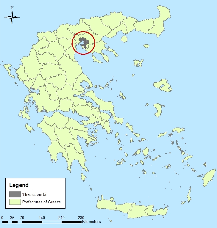 | Figure 1. The city of Thessaloniki in northern Greece |
2. Material and Methods
2.1. Selection of Data
The road that has been selected to be under study is one of the most central roads from the road network of the city, named ‘Tsimiski’. The total length of the road is approximately 1755m so it was divided into eleven segments as it is shown at figure 2, starting and ending at nodes with traffic lights. The aim is to exclude the spent time at traffic lights in order to have higher accuracy at the prediction times. For those segments, it was possible to calculate the travel time between them through GPS time data and knowing the distance of segments. At table 1 it is defined the length of each one of the eleven road segments. The length varies from 78 to 270 meters.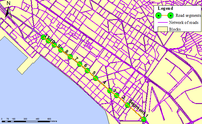 | Figure 2. Study-area: Tsimiski road and its segments, downtown Thessaloniki |
| Table 1. The 11 segments of Tsimiski road |
| | Segments’ ID | Length (m) | | 1 | 269,6727 | | 2 | 173,453 | | 3 | 97,801 | | 4 | 226,199 | | 5 | 142,8451 | | 6 | 126,08 | | 7 | 142,951 | | 8 | 138,1332 | | 9 | 102,1174 | | 10 | 90,8395 | | 11 | 78,19 |
|
|
First of all, it should be transformed the coordinates of GPS points from WGS84 the coordinate system that GPS use to Greek Grid (EGSA87). This contributes to higher accuracy of results. This was performed using one of the most common GIS software packages named ArcGIS. In addition, it should be selected from the numerous data the points that were assigned to the Tsimiski road. Thus, there were selected Tsimiski’s points giving a margin of 80 meters right and left of the road through ArcGIS. Another one excluding criterion was the vehicle’s orientation. Since Tsimiski has only one direction the points should have similar orientation. So it was defined a wide of values for the orientation and points that didn’t follow this criterion were excluded. At the following figure some of the numerous transformed points are represented. These points are already filtered by road and orientation.
2.2. Map-Matching
The data have to be referenced spatially, so a proceed of map-matching was necessary. This procedure is a crucial issue especially in urban areas as Thessaloniki with narrow roads, tall buildings and other signal degraded environments. Thus, it is challenging to identify the actual link on which the vehicle is travelling and to determine the vehicle location in that link. There are many proposed procedures for map matching varying from those using simple search techniques to those using more advanced techniques. Many of them have been used in urban and suburban areas and the percentage of correct links ranges between 86% and 93% and the 2-D horizontal accuracy range between 15m and 10.6m. [3] In this study, it has been selected one map-matching method that has been successfully accepted by the international community and it is based on the idea of using as spatial street network only the road segments which are measured by the system itself and not by external sources (i.e., electronic city maps produced by other surveying methods). The mathematical algorithms which have been used were the linear regression model and its prediction zone. The method has been tested in different confidence levels (95%, 97.5% and 99%) and in the case of standalone GPS observations gave map-matching accuracy range between 15m. and 21m. In the case of differential GPS observations the range was 1.5m to 2.0m. [5], [6]. The general mathematic model of linear regression is the following: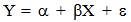 | (1) |
And its confidence interval or prediction zone for every road segment is given by the following relationship: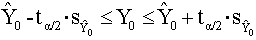 | (2) |
Normally, the prediction zone is defined by two hyperbolic curves while the most close point is defined implementing the equation (2) for x mean. However, at the current study, the difference between maximum and minimum points is so small giving the possibility to assume the hyperbolic curve as a straight line. [7] After implementing the method of linear regression a set of spatial models are revealed, each one for a segment and theirs prediction zones in meters. This means that any point of vehicle’s route located within the zone, will be matched with the regression line. The points that didn’t belong to each prediction zone were excluded as it is shown at figures 3 and 4. 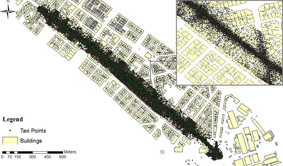 | Figure 3. Taxi points at Tsimiski road before map-matching |
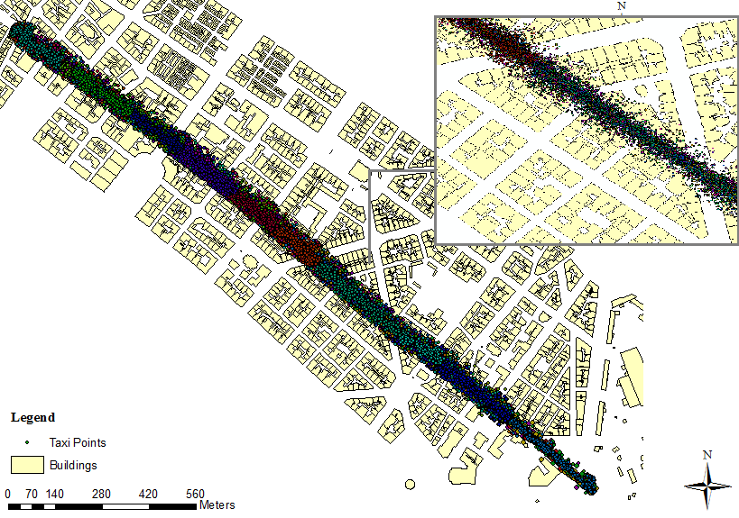 | Figure 4. Taxi points at Tsimiski road after map-matching |
| Table 2. Prediction Zone of each Road Segment |
| | Road Segment (East to West) | Spatial Model | Prediction Zone ( m) | | 1 | y=55,564-0,6508*x | 24,3409 | | 2 | y=54,67-0,61185*x | 46,3591 | | 3 | y=52,533-0,51871*x | 33,8955 | | 4 | y=55,545-0,64996*x | 38,4413 | | 5 | y=54,697-0,6130*x | 40,5247 | | 6 | y=53,808-0,51871*x | 43,3335 | | 7 | y=52,533-0,57426*x | 42,06263 | | 8 | y=52,784-0,52964*x | 33,3642 | | 9 | y=52,311-0,50904*x | 34,2593 | | 10 | y=52,603-0,52175*x | 37,5229 | | 11 | y=52,782-0,52955*x | 37,76667 |
|
|
2.3. Calculation of Travel Times
At this stage, it was feasible to calculate travel times per road segment during all the day for every single day. The implementation was performed through the mathematical software Matlab because the numerous data constituted a critical problem. The process of calculation was performed as following:• Identify TAXI’s ID that is appeared among the road segment at least twice in order to be possible to calculate its travel time• Select points with same ID at the same period of day• Calculation of travel time from point p to p+1• Exclude travel times with more than some minutes depending on each segment’s length. For instance a travel time more than 4 minutes for 200m indicates that the vehicle had a different route• Calculation of travelled distance and a further calculation of time travel in relation with the segment’s length.
2.4. Travel Time Prediction
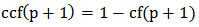
Having the travel times, a travel time prediction is possible. The method of Kalman Filter was performed through Matlab. Kalman Filter is a set of mathematical equations that implement a predictor-corrector type estimator [8]. The basic typology of this method is the following:If p the place where the vehicle is situated• cf the contribution from filtering• cca the contribution from the cycle action• e the error of filtering• P the prediction• rtpv(p) the Real Time of Previous vehicle• rtpd(p+1) the Real Time of Previous Day • var3d the Variance of the 3 last Days• varP the prediction’s variance• rtday1(p+1), rtday2(p+1), rtday3(p+1) real time of vehicle the previous day, 2 days ago and 3 days ago respectively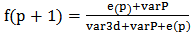 | (3) |
 | (4) |
 | (5) |
 | (6) |
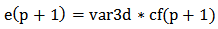
Taking into consideration the admission that var3d=varP the equation (3) is transformed as following [1]: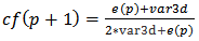 | (7) |
The whole process is briefly described at the following figure where it is obvious that the process is a loop consisted of two basic steps. The first step is “Measurement Update – Correction” and the second step “Time Update – Prediction”. The procedure is repeated for each time step using the state of previous time as an initial value. Therefore the Kalman Filter is called a recursive filter. [4]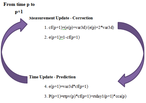 | Figure 5. Kalman Filter Loop |
3. Results and Discussion
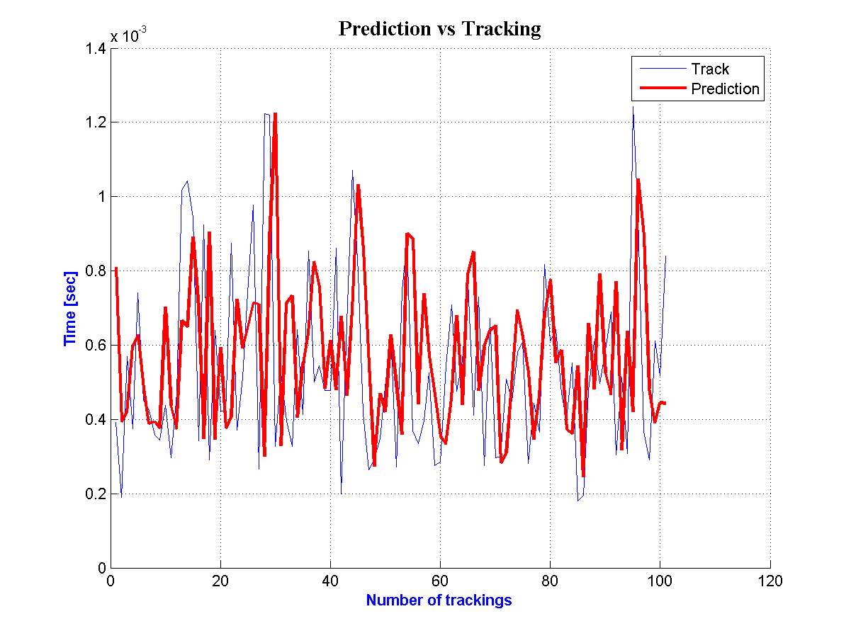
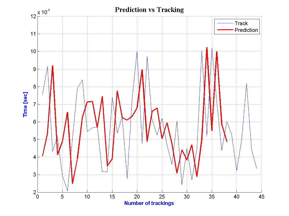
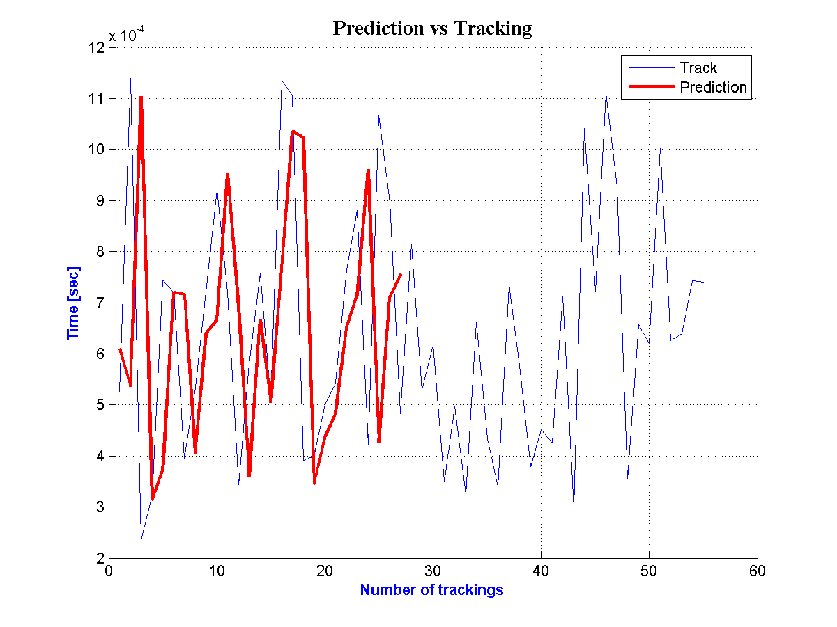
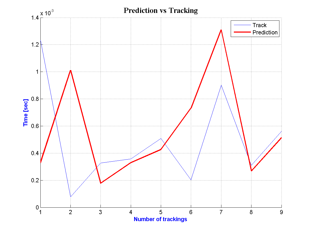
After implementing the above method a great amount of results are created. For each one day it has been created a comparative diagram between prediction travel time and tracking through Matlab. At the following diagram it is shown this comparison for one day at 1st road segment for almost 90 vehicles. It is easily noticed a satisfactory performance of the above method.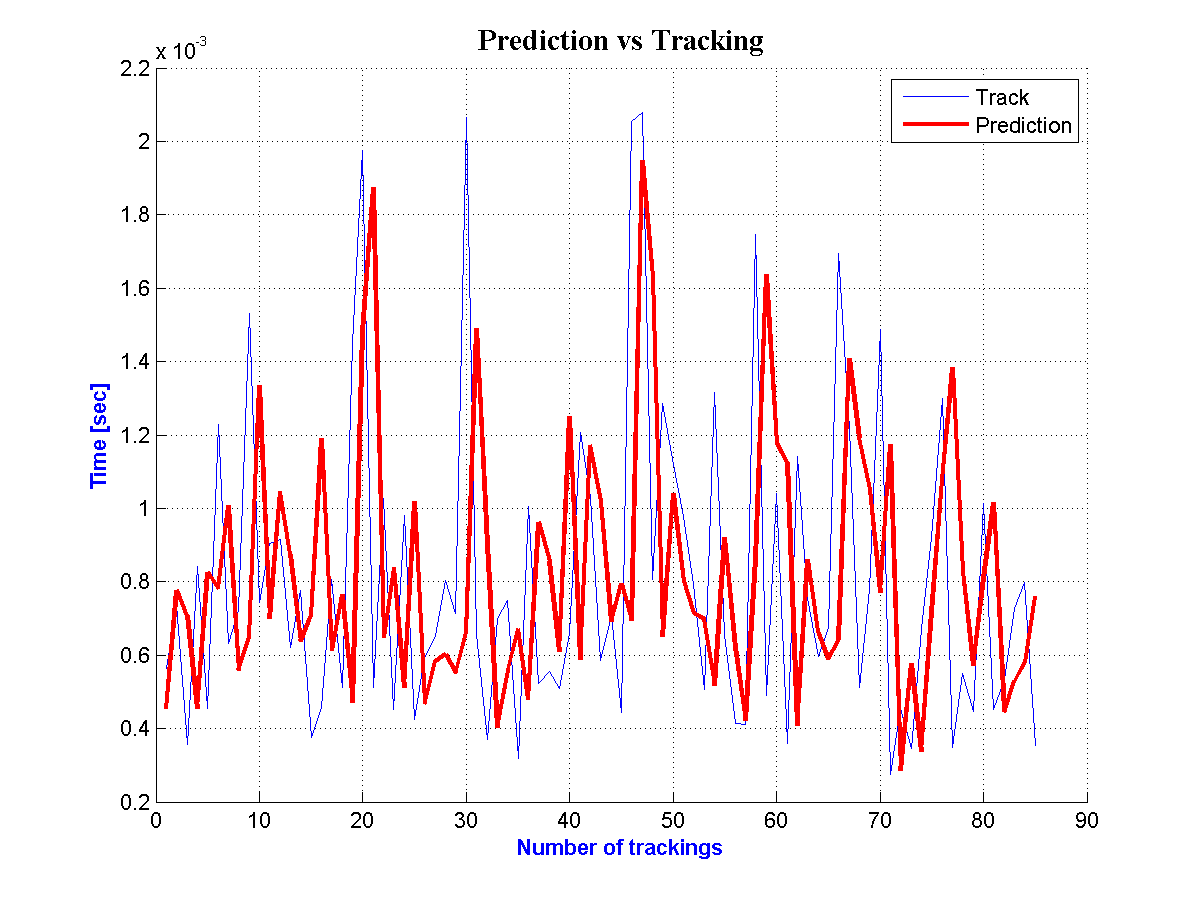 | Figure 6. Prediction and Tracking for the  Road Segment Road Segment |
 | Figure 7. Prediction and Tracking for the  Road Segment Road Segment |
 | Figure 8. Prediction and Tracking for the  Road Segment Road Segment |
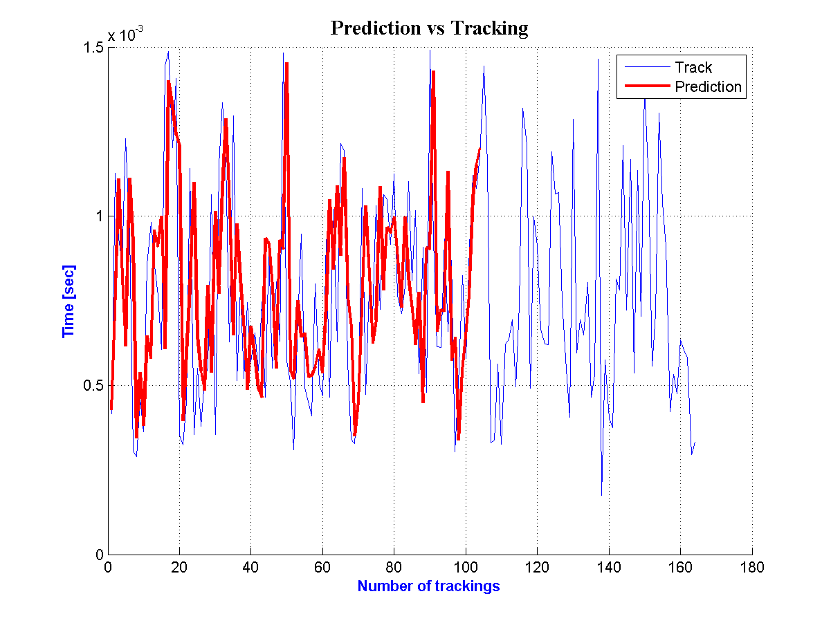
The same efficiency is observed at the figures 6 and 7 for the second and third road segment where there are predictions for 100 vehicles per road segment respectively.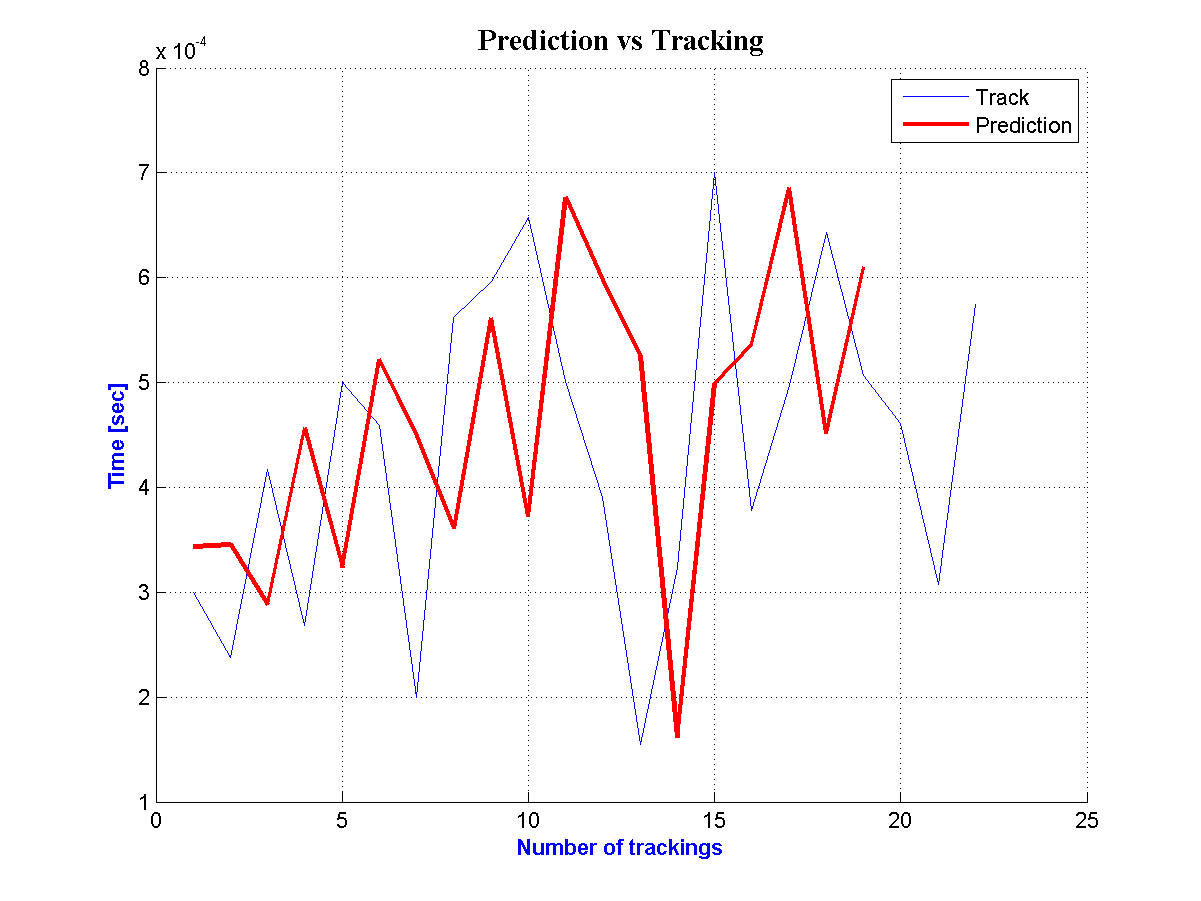 | Figure 9. Prediction and Tracking for the  Road Segment Road Segment |
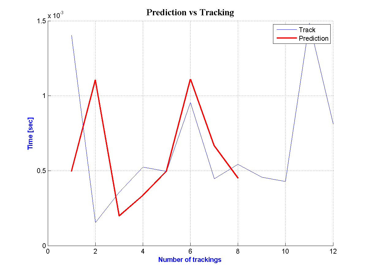
It should be referred that there isn’t the same number of predictions for each road segment per day because many GPS points have been excluded at previous phases.For the same reason at the three followings figures the number of predictions is restricted, consequently, the difference between prediction and tracking is intensively augmented.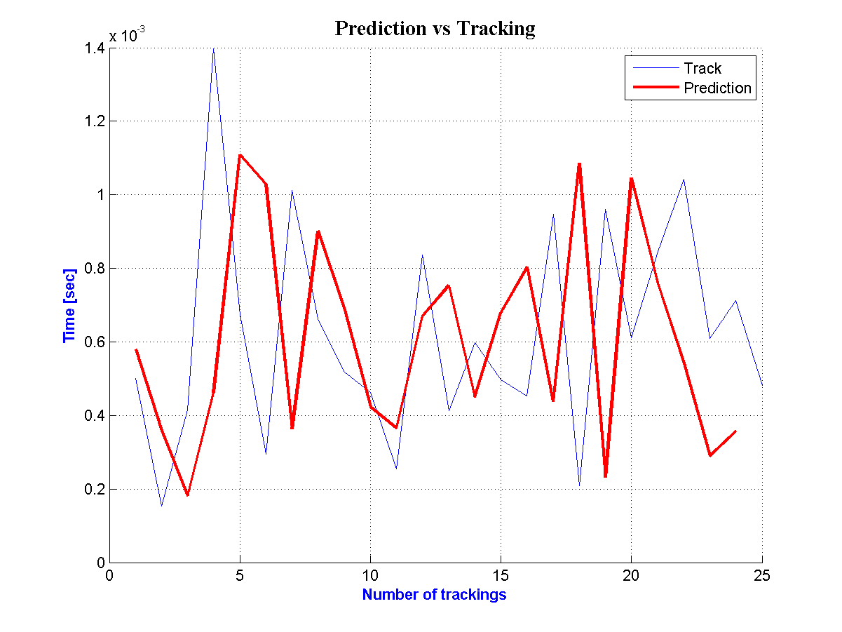 | Figure 10. Prediction and Tracking for the  Road Segment Road Segment |
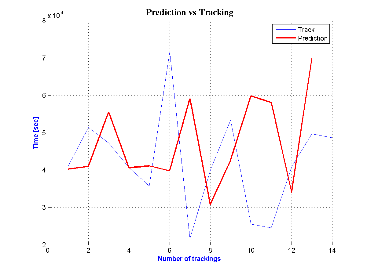 | Figure 11. Prediction and Tracking for the  Road Segment Road Segment |
 | Figure 12. Prediction and Tracking for the  Road Segment Road Segment |
 | Figure 13. Prediction and Tracking for the  Road Segment Road Segment |
At the three last figures which concern the three last road segments the predictions are a few because the road segments are too short. In addition, if there is at least one day with few GPS points the number of predictions is immediately decreased. So the GPS points are limited particularly after implementing the excluding criteria. As a result the following figures are not representative. 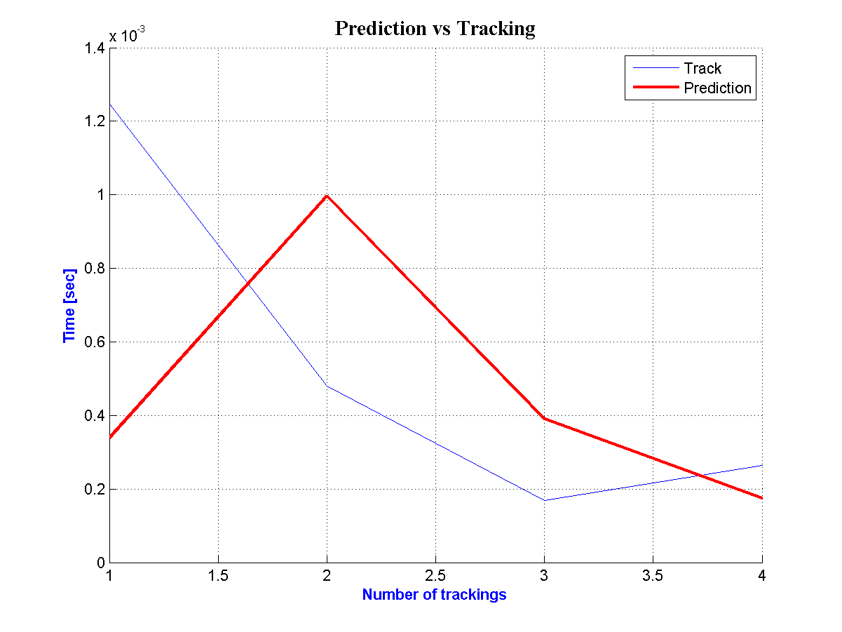 | Figure 14. Prediction and Tracking for the  Road Segment Road Segment |
 | Figure 15. Prediction and Tracking for  Road Segment Road Segment |
 | Figure 16. Prediction and Tracking for the  Road Segment Road Segment |
The table 3 constitutes a sample of prediction and tracking times for the first road segment and 4 days for 40 taxi-vehicles.| Table 3. Predictions and Tracking times for the 1st Road Segments and for the first 4 days |
| | Day | 1 | 2 | 3 | 4 | | Vehicle | Prediction | Tracking | Prediction | Tracking | Prediction | Tracking | Prediction | Tracking | | 1 | 0:01:00 | 0:01:05 | 0:00:53 | 0:00:41 | 0:00:42 | 0:02:17 | 0:01:25 | 0:01:11 | | 2 | 0:00:59 | 0:00:41 | 0:00:41 | 0:00:54 | 0:02:03 | 0:00:47 | 0:01:10 | 0:02:17 | | 3 | 0:01:34 | 0:01:20 | 0:01:05 | 0:01:12 | 0:01:00 | 0:00:59 | 0:01:44 | 0:01:28 | | 4 | 0:01:19 | 0:00:18 | 0:01:07 | 0:01:16 | 0:01:04 | 0:00:55 | 0:01:12 | 0:02:03 | | 5 | 0:00:51 | 0:01:44 | 0:01:29 | 0:01:23 | 0:00:59 | 0:00:28 | 0:01:22 | 0:01:51 | | 6 | 0:01:28 | 0:01:29 | 0:01:25 | 0:01:20 | 0:00:46 | 0:02:07 | 0:01:56 | 0:00:45 | | 7 | 0:01:55 | 0:00:45 | 0:01:03 | 0:01:44 | 0:01:56 | 0:00:31 | 0:00:39 | 0:00:46 | | 8 | 0:01:08 | 0:00:23 | 0:01:12 | 0:02:39 | 0:01:28 | 0:02:07 | 0:01:24 | 0:02:21 | | 9 | 0:00:27 | 0:02:23 | 0:02:33 | 0:01:43 | 0:01:59 | 0:01:20 | 0:02:08 | 0:01:08 | | 10 | 0:02:14 | 0:00:47 | 0:01:27 | 0:02:41 | 0:01:51 | 0:00:45 | 0:00:57 | 0:02:24 | | 11 | 0:00:49 | 0:01:20 | 0:02:35 | 0:01:33 | 0:00:49 | 0:02:00 | 0:02:21 | 0:00:40 | | 12 | 0:01:16 | 0:02:36 | 0:02:04 | 0:02:36 | 0:02:17 | 0:01:04 | 0:00:51 | 0:00:28 | | 13 | 0:01:47 | 0:02:22 | 0:02:31 | 0:01:25 | 0:01:12 | 0:01:00 | 0:00:39 | 0:00:57 | | 14 | 0:02:03 | 0:01:33 | 0:01:26 | 0:00:58 | 0:00:59 | 0:00:39 | 0:00:52 | 0:01:03 | | 15 | 0:01:41 | 0:00:37 | 0:00:48 | 0:01:14 | 0:00:54 | 0:01:21 | 0:01:09 | 0:00:45 | | 16 | 0:01:21 | 0:01:39 | 0:01:25 | 0:01:50 | 0:01:28 | 0:00:44 | 0:00:44 | 0:00:49 | | 17 | 0:01:24 | 0:00:32 | 0:01:17 | 0:01:58 | 0:01:18 | 0:01:40 | 0:01:11 | 0:00:44 | | 18 | 0:00:35 | 0:00:17 | 0:01:42 | 0:02:51 | 0:02:13 | 0:01:00 | 0:00:51 | 0:00:42 | | 19 | 0:00:33 | 0:02:54 | 0:02:53 | 0:02:43 | 0:01:38 | 0:00:37 | 0:00:40 | 0:02:13 | | 20 | 0:02:29 | 0:01:45 | 0:02:31 | 0:00:38 | 0:00:37 | 0:01:30 | 0:02:04 | 0:00:46 | | 21 | 0:01:34 | 0:01:01 | 0:00:43 | 0:00:50 | 0:01:27 | 0:01:16 | 0:00:49 | 0:01:26 | | 22 | 0:01:40 | 0:01:50 | 0:01:14 | 0:01:34 | 0:01:24 | 0:01:06 | 0:01:17 | 0:01:25 | | 23 | 0:01:43 | 0:01:14 | 0:01:26 | 0:01:02 | 0:01:05 | 0:00:29 | 0:01:02 | 0:01:31 | | 24 | 0:00:57 | 0:00:58 | 0:01:00 | 0:01:16 | 0:00:49 | 0:01:05 | 0:01:26 | 0:01:12 | | 25 | 0:01:02 | 0:01:24 | 0:01:18 | 0:00:28 | 0:00:49 | 0:00:49 | 0:01:01 | 0:01:44 | | 26 | 0:01:22 | 0:00:55 | 0:00:40 | 0:00:39 | 0:00:46 | 0:01:34 | 0:01:40 | 0:00:37 | | 27 | 0:00:54 | 0:02:08 | 0:01:14 | 0:00:30 | 0:01:04 | 0:01:02 | 0:00:49 | 0:02:12 | | 28 | 0:01:58 | 0:02:25 | 0:01:21 | 0:01:15 | 0:01:07 | 0:00:50 | 0:01:40 | 0:00:58 | | 29 | 0:01:42 | 0:02:31 | 0:01:46 | 0:02:05 | 0:01:18 | 0:01:13 | 0:01:03 | 0:00:42 | | 30 | 0:01:51 | 0:02:50 | 0:02:23 | 0:01:29 | 0:01:20 | 0:01:17 | 0:00:57 | 0:01:18 | | 31 | 0:02:48 | 0:01:43 | 0:01:34 | 0:01:28 | 0:01:20 | 0:01:38 | 0:01:19 | 0:00:57 | | 32 | 0:01:42 | 0:00:37 | 0:01:26 | 0:00:35 | 0:01:36 | 0:02:34 | 0:01:46 | 0:01:53 | | 33 | 0:00:54 | 0:02:04 | 0:01:19 | 0:00:41 | 0:01:38 | 0:00:34 | 0:01:26 | 0:02:00 | | 34 | 0:01:38 | 0:01:43 | 0:01:04 | 0:01:47 | 0:00:58 | 0:01:53 | 0:02:00 | 0:01:48 | | 35 | 0:01:30 | 0:01:21 | 0:01:46 | 0:00:57 | 0:01:44 | 0:01:04 | 0:01:27 | 0:00:30 | | 36 | 0:01:08 | 0:00:57 | 0:00:57 | 0:02:24 | 0:01:43 | 0:00:31 | 0:00:31 | 0:00:49 | | 37 | 0:01:02 | 0:01:20 | 0:02:17 | 0:00:38 | 0:00:33 | 0:00:46 | 0:00:48 | 0:01:14 | | 38 | 0:01:19 | 0:01:56 | 0:01:15 | 0:01:21 | 0:01:01 | 0:00:31 | 0:00:55 | 0:01:34 | | 39 | 0:01:40 | 0:00:46 | 0:01:07 | 0:00:38 | 0:00:33 | 0:00:41 | 0:01:33 | 0:00:51 | | 40 | 0:00:46 | 0:00:20 | 0:00:36 | 0:00:40 | 0:00:41 | 0:00:31 | 0:00:42 | 0:01:15 |
|
|
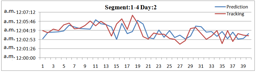
Trying to investigate the effectiveness of the whole method it is compared the prediction and tracking time for more than one road segment simultaneously. The results are presented at following figures. At the four following figures it is compared the travel times for the first 4 road segments for 4 days respectively and 40 vehicles. The results are quite positive concerning the effectiveness.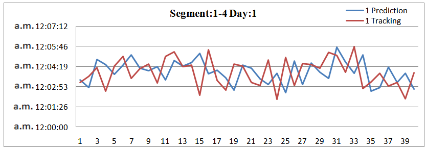 | Figure 17. Prediction and Tracking for 4 road segments and 40 vehicles |
 | Figure 18. Prediction and Tracking for 4 road segments and 40 vehicles |
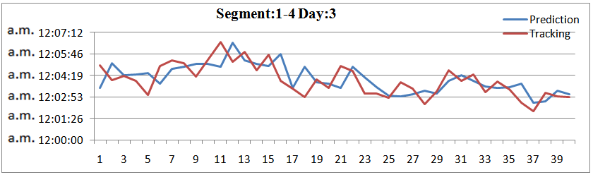 | Figure 19. Prediction and Tracking for 4 road segments and 40 vehicles |
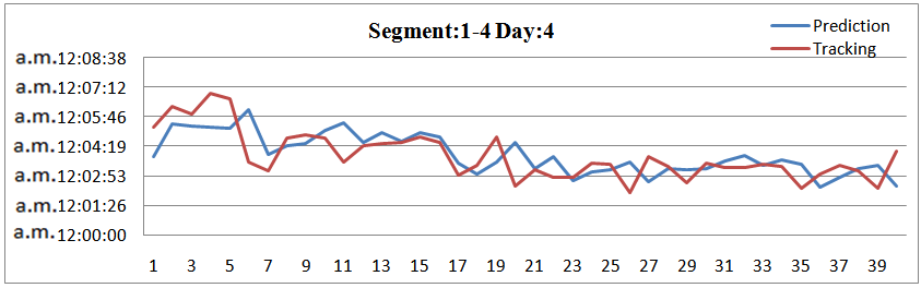 | Figure 20. Prediction and Tracking for 4 road segments and 40 vehicles |
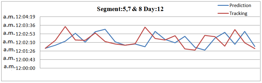
The 3 figures below concerns the road segments 5,7 and 8 presenting the difference between prediction and tracking times for 25 taxis vehicles and 3 days respectively. It must be noted that some road segments are not selected for this comparison because of the restricted number of predictions times that make impossible the comparison.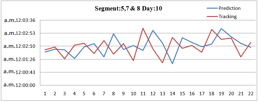 | Figure 21. Prediction and Tracking for 3 road segments and 25 vehicles |
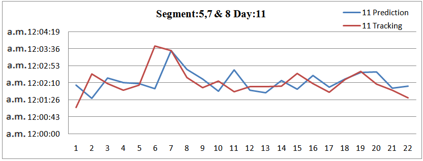 | Figure 22. Prediction and Tracking for 3 road segments and 25 vehicles |
 | Figure 23. Prediction and Tracking for 3 road segments and 25 vehicles |
4. Conclusions
The benefits of an efficient traffic prediction system are very significant. This system can affect positively many sections such as social, environment and of course economy. First of all, traffic predictions are very important as they enable to detect potential traffic jam spots. So, the local stakeholders based on the information provided from the traffic prediction system can initiate certain traffic control methods to avoid the traffic jams. Furthermore, it is a precious tool which indicates the weaknesses of the road network providing with knowledge about where it is crucial to improve the infrastructures. This system could also be used as a tool for urban planning in the city defining the land uses according to traffic congestion spots. For instance, roads such as Tsimiski Street are inconvenient for residence because of the continuous noise and air pollution, while, on the contrary, this road is suitable for commercial uses. This traffic prediction system could also help to increase the safety on the roads by diminishing the number of injury accidents. The combination of the methods that are used in the current study can be assumed as an effective process to predict travel times in a dense urban area such as Thessaloniki city. In addition, the process uses the least possible equipment without negative effects to everyday operation of the city. However, a significant condition for an effective performance of the whole method is the existence of over 20 GPS points per road segment per day. In case of fewer, the errors’ wide might be over 90 seconds. The basic requirements for the study are the computational and processing strength and a large amount of GPS points. So, it constitutes a cost-effective endeavor to mitigate a crucial problem that degrades the life’s quality and deteriorates day by day.The endeavor to automate the process is also successful since each stage of the current study was performed through programming in Matlab. Without programming, the process would be quite difficult to be implemented because of numerous data. So the whole process contributes to one integrated and smart traffic prediction system. A further study could be performed taking into consideration the peak periods of every single day in order to investigate whether the method will be ameliorated or not. At future studies it would be also interesting to incorporate the field of vehicles’ velocity in the process of Kalman Filter. Finally, it would be also interesting to investigate the efficiency of a traffic prediction system using different method such as fuzzy logic, exponential smoothing, and artificial neural networks et-c. The result could be compared among them and Kalman filter method in order to investigate the most effective combination of methods.
References
| [1] | Daskalakis Nikolaos, "Telematics systems using GPS for mass transit vehicles & pattern predictions in real time", diploma thesis, 2008. |
| [2] | Gidófalvi Gyozo and Morán Carlos, "Estimating Traffic Performance in Road Networks from Anonymized GPS vehicle Probes", in Proceedings of Workshop on Movement Research: Are you in the flow? at the 13th AGILE International Conference on Geographic Information Science, 2010. |
| [3] | Kim Wuk, Jee Jee Gyu-In and Lee JangGyu, "Efficient use of digital road map in various positioning for ITS", in Proceedings of IEEE Symposium on Position Location and Navigation, San Diego, CA.,pp.170-176, 2000. |
| [4] | Kleinbauer, “Kalman Filtering Implementation with Matlab Study Report in the Field of Study,” November, 2004. |
| [5] | Lakakis Konstantinos, Savvaidis Paraskevas, Ifadis Ioannis, Doukas Ioannis, "Quality of Map-Matching Procedures Based on DGPS and Stand-Alone GPS Positioning in an Urban Area", in Proceedings of International conference, FIG Working Week 2004 Athens, Greece. |
| [6] | Lakakis Konstantinos, Savvaidis Paraskevas, "Map-Matching Procedures at Urban Grade Intersections", in Proceedings of “10th International Conference on Applications of Advanced Technologies in Transportation (AATT2008)”, Athens, Greece. |
| [7] | Lakakis Konstantinos, "Land Vehicle Navigation in an Urban Area by Using GPS and GIS Technologies", PhD Dissertation, Aristotle University of Thessaloniki. |
| [8] | Yunlong Zhang and Zhirui Ye, "Short-Term Traffic Flow Forecasting Using Fuzzy Logic System Methods", Taylor & Francis, Journal of Intelligent Transportation Systems, 12:3, pp.102-112, 2008. |
 Abstract
 Reference
 Full-Text PDF
 Full-text HTML