1. Introduction

Within GIScience advances, methods to explore spatial patterns in Geographic Information System (GIS) networks remain vacuous. Fischer and Curtin expose the vantage in the research of networks because it represents exceptionally complex systems[1, 2]. These complex systems, or networks, support life as we know it on Earth. Illustrations of these complex systems include transportation systems, utilities, rivers and streams. Spatial patterns sought within these complex systems are defined as; "an object, or between objects that is repeated with sufficient regularity" [3]. The objective of this research is to consider new empirically tests for a new method for spatial patterns in GIS networks.

Prior advances in non-spatial network pattern research disregards important aspects for understanding geographic location[2, 4, 5]. Examples of non-spatial network pattern analysis techniques primarily rely on connectivity and topological relationships, rather than geographic properties [6, 7]. Network metrics that are used to find patterns, do not embrace the spatial dimension[8, 9].

Conversely, strategies for identifying spatial patterns in GIS networks have been explored. Many of these strategies have been empirically developed to identify patterns in road networks only[10, 11, 7, 12, 13]. The opportunity is therefore provided for research on other spatial network phenomena.

Previous research also demonstrates strategies that isolate only a few pattern types. These limited pattern types are: grids[10, 7, 13], strokes[14], ring roads[15], and star patterns[14, 3]. Although these are important road network pattern identification methods, they are highly sensitive to variations in the data, are computer processing intensive, and deductively work on only one pattern type at a time[10, 7, 13, 14, 15, 3]. In a practical setting, pattern types may not be known at the time of investigation, and a more inductive approach may be beneficial.

Many networks are dynamic and change over time. As examples, new roads are constructed, rivers change course, and utility systems are expanded. Research to date on network patterns consider only a single temporal representation. By considering only a single point in time, the representation of the network systems, their patterns, and our understanding how the patterns change is limited.

The method presented for consideration in this research will be GIS based and inductive. The method will work regardless of the spatial networks they model, the pattern types identified, and embrace multiple time series for analysis. The proposed method is called DAS. DAS stands for the variables of features that will be used to derive a single quantitative metric for pattern detection. D, stands for density, and will measure the density of nodes within the target geographic dataset. A, stands for angles, and will measure the edge angle for features. S, stands for shape and will be a calculated value for polygons that are inherent with networks for areas enclosed by the edges. The DAS method will be tested against specific non-spatial network measures, geographic phenomena, pattern types, and human cognition.

To help improve the understanding of spatial patterns in GIS networks, the DAS method will make four contributions. One, the DAS method will run in GIS and focus on the spatial aspects of networks for pattern identification. "To ignore it (spatial aspects of a network) is to miss some of these systems' (spatial networks) most interesting features"[16]. Two, DAS will be analyzed against more phenomena types than roads. Three, the DAS method be analyzed against more pattern types than the grid, stroke, ring road, or star pattern. Fourth, the DAS method will be used to analyze more than a single temporal network dataset.

2. Background

Networks are a series of connected vertices or nodes and edges or lines. "Network data structures for geographic information science (GISci) are methods for storing network data sets in a computer in order to support a range of network analysis procedures"[1]. Curtin also points out that a network can represent a transportation or communications system, a utility service mechanism, or a computer system, to name only a few network applications" [1]. Types of networks include flow networks and pure networks. Fischer, explains flow networks will contain information on the flow of something within a network and a pure network represents any networks overall structure where the main concern are the topological relationships [17]. Additional examples of networks include computer networking, social networks, utility networks, hydrology networks, and the list goes on. Critical is the idea, that a network by definition can be used to model and analyze linear features and their relationships.

The elements used to make up a network, nodes (points or junctions) and edges (lines or arcs) form the basis in GIS network models. Notably, as Curtin points out, one of the earliest GIS representations used network data structures [18]. The underlying intent of networks is, "to help us understand or predict the behaviour of these systems"[6].

The theoretical basis for networks, network models and network analysis comes from principles in mathematics, topology, and graph theory[18, 6]. Important contributions from graph theory are discuses in the next section and provides the foundation for characterizing networks, network analysis, and network patter analysis.

A simple graph consists of the following objects G = (V,E). In this example, G is the graph and V is the vertices (points) and E are the edges (lines). A model such as this is often depicted in the form of a picture. Figure 1, provides an example of a simple graph where there are three vertices and three edges. As a principle, vertices do not loop back upon themselves[19]. The first noted example of problem solving using graph theory was written in 1736 by Leonhard Euler. In this seminal article he used a graph to solve the Königsber Bridge Problem. In his writings, he found a solution for using seven bridges connecting two islands to the banks and one another. The problem was to traverse each bridge once without doubling back. Interestingly, he proved using graph theory that a solution to the problem did not exist[19]. Since the time of Euler graph theory and its applications has evolved. Today, network modeling persists based on the same basic principles used by Euler, however, with the advent of computers and GIS the amount of information that can be modeled and the complexities of the systems has increased. For a more in depth review, Newman's 2003 article, "The Structure and Function of Complex Networks" is recommended[6].

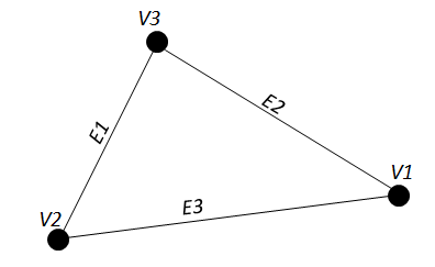
Figure 1. A simple graph

Graph descriptions of networks are a logical way to characterize a network. For example the Tree or Branching networks are often used to model streams or hydrological systems. The Manhattan network, is a network constructed with 90 degree angles between edges. These are often seen in city blocks of road networks. A couple of additional examples include the bipartite graph, and the hub and spoke[1].

Graphs can also be described based on more quantitative measures. Scientists often analyze the total number of edges and vertices within a network. They may also provide the degree of the vertices expressing the number of coincident edges[18]. Other quantitative measures rely on calculations or indices for a network. Curtin explains that the simplest is called the Beta Index. The Beta Index provides a result built upon the networks number of edges over the number of vertices. Another measure is called the Alpha Index that compares the "maximum number of fundamental cycles in the graph to the actual fundamental cycles in the graph"[18]. A final example is called the Gamma Index, where the number of possible edges in a graph are compared to the actual connections represented. These various metrics and indices provide scientists with the fundamentals to share information about their graphs or networks with others in a meaningful way.

Networks that represent geographic features have extended the options for characterizing graphs when used in a map or GIS. According to Gaster, "Interest in the spatial structure of networks dates back to the economic geography movement of the 1960s"[5]. Kansky, is noted for his work in his Doctoral Thesis where he initiated the modern discussion of road network structures[20]. Marshall, extended the discussion on the structure of roads and streets and developed a descriptive taxonomy for road networks[20].

Another important characterization of networks lies in the relationships within a network. These include a network's density, heterogeneity, connectivity, accessibility, interconnectivity, entropy, and even the connection patterns [13]. The use of these elements has received the attention of geographers in analyzing issues dealing with networks and problem solving. By using these measurable elements Fischer notes GIS and network analysis are "burgeoning fields" of study[2].

With the explosion of social media, spatial network analysis methods have also been applied to the geography of instant news messaging such as Twitter[21]. Takhteyev analyzed 481,248 tweets by geocoding the locations of the users and then applied regression analysis nodes representing the 25 largest regional clusters of users[21]. Edges were assigned with weighted variables and distances could be assessed. The results empirically showed that an overwhelming majority of tweeting is done within a small geographic area. The authors of this study "highlight the importance of considering structural constraints on ties rather than simple distance"[21]. In other words, the spatial consideration for network analysis of social networks does not provide a full picture and additional considerations such as patterns in the networks themselves should also be further studied.

There are numerous strategies and methods that have been used for pattern identification and analysis on transportation networks[10, 12, 13, 22, 9, 4, 3]. One example is where Yang applied a four step methodology for isolating grid patterns in road networks. Yang's first step required the building of topology for roads and intersections, and then to generate polygons contained within the roads themselves[10]. The second step was to generate values for parameters like consistent arrangement, shape similarity, and grid shape index were calculated. The third step uses a multi-criteria decision problem solution to adaptively assign thresholds to each parameter. This multi-criteria decision problem solution is called CRITIC and was developed by Diakoulaki, Mavrotas, and Papayannakis[23, 10]. The final step resolves grid patterns incrementally with an algorithm. Although successful in isolated the grid patterns in the study areas, Yang's study argues that the grid patterns are the only focus because they are most common. Since patterns take the form of more than just grids, further expansion of this method would be needed to apply the study more broadly[10].

Similarly to the study of Yang et al., Usui[8] proposes a method to evaluate patterns in road networks. Usui and Asami's purpose for analyzing the road network patterns was to isolate illegal fire-inextinguishable areas (FIA) within cities. The approach considers "well laid out roads" to test conformity to tree, grid, and delta patterns. Using graph theory principles such as grid-tree-proportion index (GTP), alpha index and gamma index, the author is able to make some pattern identification comparisons. The ratio of the actual road links to the maximum number of links is the gamma index value. Applying this analysis on the Bunkyo ward in Tokyo, Japan, results in challenges in working with scale and boundary definition errors. A step to limit the area of analysis to a radius is added that resolves these challenges. In the end the author is successful in defining a pattern analysis method for isolating areas in Tokyo, Japan that are out of compliance with FIA. However, issues in scale and pattern isolation more broadly remain unsolved.

Marshall's taxonomy of road network structures includes linear, tree, radial, cellular and hybrid forms[20]. The patterns that have gained the highest amount of attention include "strokes as type of linear forms, grids as type of cellular forms, stars as type of radial forms and circular roads as type of cellular forms"[10, 11, 7, 24, 22]. Detection and quantification of these patterns have been approached through many strategies. A presentation of how to approach each pattern was presented by Heinzle et al.[24].

Table 1. Pattern Detection Approaches

GIS Shape Analysis

In a GIS or simply on a paper map, phenomena are often represented by delineating or segregating areas from one another using boundary lines. These lines, when enclosed form polygons. These polygons have shape. "Shape has always been of concern in geography"[25]. Measuring shape is critical in order to make meaningful comparisons and detect potential patterns across geography. Taking this one step further, "Measuring shape, that is, quantitatively describing the geometric form of a closed homogenous region, is frequently used to better understand spatial processes at work in the landscape[26]. A wide range of research on the topic of shape has been conducted. Fields such as physics[27] forensics[28], biogeography[29], and mathematics[30] are just some of them. Others include facial recognition[31], database mining, and computer image retrieval systems. Although the identification of a shape may seem intuitive, the synthetic training of a system is actually quite complex.

Shape Cognition

Shapes, identified in maps by humans, hold an important role in geography[32, 33]. In a study by Sanders and Porter, they demonstrate that an individual's "mental map" is based on ideal shapes and there are statistical errors humans naturally make in terms of orientation and size when comparing a participant's mental map to an actual map. These results tip the hand towards GIS as a quantitative means to reproduce shapes and maps repeatedly without human natural tendencies towards error such as orientation. This means using GIS would appear to be the simple way to proceed with shape analysis in geography. Linework insides' become bound yardsticks. Shapes uncover certain kept secrets. Unfortunately, this line of thinking can actually be quite complex[26]. Regardless, the value of quantitative measures for scientific purposes is critical as the mental map of one person will most certainly differ from person to person. In the modern era of GIScience, Montello argues, "further research into human cognition with geographic information and GIS makes sense and seems valid"[34]. This is an agreeable position, as the need for scientifically repeatable systems are needed for problem solving. Montello further states that "good cognitive research is difficult"[34]. With the understanding that cognitive research is difficult, cognitive shape identification within the methods of this research will be addressed with deliberate concern.

Quantitative Shape Measures in Geography

Determination of meaningful measures for shape in geographic phenomena have appeared in geography research since the 1960's[35, 26, 36, 37, 25]. "Shape indices tend to fall into two classes: single parameter, such as area or perimeter calculations, and multiple parameter, involving more complex mathematical functions"[26]. A noteworthy theoretical construct that has been adopted by geographers is Christaller's Central Place Theory (CPT). Through Christaller's observation of settlements and towns he theorized an ideal surface laid with hexagon shapes. The hexagon's geometrically perfect in the sense that no space is technically wasted. As a theory, Christaller's hexagon model is ideal. In practicality, settlements of cities and town do not follow this ideal shape. To study irregular shapes and settlement, another approach was needed. The need for a quantitative measure of shapes that could address phenomena as they exist would come with the quantitative revolution in the 1960's. One approach that emerged was conceived by William Bunge and was presented in his work, Theoretical Geography[38]. In his approach, he deconstructs the polygons of ninety-seven irregularly shaped Mexican communities by using "vector lag measurements". Bunge's work was later improved upon by Boyce and Clark. The desire was expressed that improving on shape methods would help us better understand urban form, trade areas, political areas, and physical features. Like Bunge, Boyce and Clark[25] presented a method for analyzing and mathematically deconstructing a polygon’s shape. How? The alternative's advantages included the ability to manage boomerang shapes and radials. The key difference was to measure a shape from a central location. This meant that scientists were no longer limited to deconstructing polygons with at least eight sides.

Analysis of Shapes in GIS

The challenge of formulating measurable indices or metrics for shapes in GIS is not due to a lack of GIS data, computer system performance or GIS software and algorithms. There's an abundance GIS data available, computer hardware performance continues to improve at astonishing rates (especially with distributed processing and cloud hosted capabilities), and options of software and methods for giving shapes a numerical identity are abundant. The challenge for measuring shapes in GIS is that there has not been an agreed upon single metric or indices for analysis[35, 39, 26]. As an example, the measure of polygon compactness in GIS has been discussed by Angel et al. and MacEachren[35, 36]. Both found there to be multiple possibilities for computing a shapes compactness[35, 36]. Research by Angel et al. specifically identified ten optional measures of shape compactness. These measures are shown in the table below and each one has a slightly different dimension in terms of what is actually being measured. Angel et al.'s descriptions are included to provide the wide range of compactness measures:

An objective of this research trajectory includes not just shape analysis but the isolation of patterns. Patterns depend on shapes as the building blocks. Due to many options in shape metrics, testing to determine the appropriate metric is required[35]. "Pattern alone is highly complex, but the measurement of shape in the context of pattern provides a mechanism to simplify pattern into basic units"[40]. A theoretical revolution in GIS for moving shape analysis forward may be required to assess the options that are available to explore along with the various applications and geographic phenomena that retain explicit shape information. This work has begun. Wentz tested a method that uses polygons' elongation, edge and perforation characteristics to detect patterns[26]. Atwood and Wentz perform another approach using polygons' Orientation, size, shape and type empirically tested on landuse and soils. Here the shape analysis was solved as an index using perimeter-to-area ratio[41]. Yang et al. use GIS shape analysis to assist with isolating grid patterns in a road network. Orientation and shape similarity measures are instrumental to the methods tested[10]. Shape analysis, due to the geometric and spatial fundamentals, provide impetus to GIScience for new methods and empirical testing[42]. On equal footing, the analysis of shape in GIS will need to model changes over time as well for a more perfect representation.

Table 2. Compactness Types for Polygons

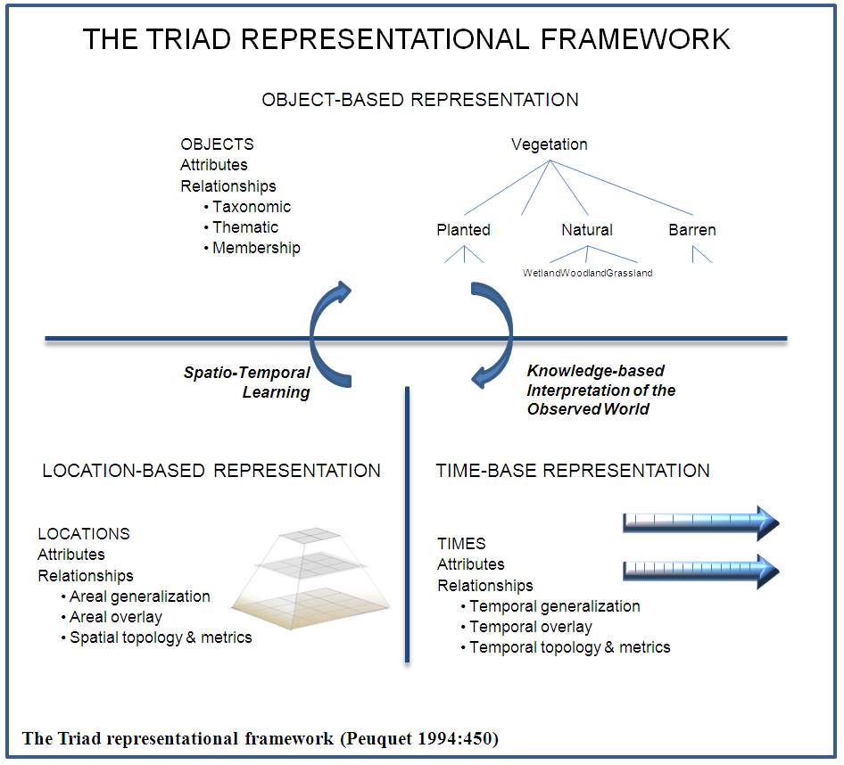
Figure 2. The Triad Representational Framework by Donna Peuquet[43]

Space and Time Geography

Looking at the dimension of time over space is a challenge today in GIS where the theoretical basis for much of space-time GIS, dates back to fundamental principles established by Newton, Einstein and ancient debates dating all the way back to ancient Greek philosophy[43]. A great number of innovative theories and approaches to modeling both space and time in GIS have evolved over the past 50 years. They tell us that modeling phenomena in space is difficult, and modeling space and time is very difficult. Special consideration of how time is modeled with space using GIS includes constraints such as continuous and discrete as well as concepts in scale. Significant space-time GIS contributions have come from Hägerstrand, Miller, Livingstone, Kwan, Peuquet and others[44, 45, 46, 47, 43, 48, 49]. Hägerstrand's conceptual framework visually demonstrated human activity constraints using space-time prisms. Hägerstrand and Miller both extended techniques to include relations in higher dimensions[44]. Kwan and Lee also extended geovisualization methods where gender/ethnic differences in space-time activity patterns reside in Portland, Oregon[46]. Donna Peuquet has advanced theory regarding space-time GIS by means of a practical model and a series of space and time concepts, constraints, and a taxonomy. The current status of GIS, can be gleaned from her comment, “Although maps may be used to depict change or movement, they have mainly been used to present a static view of the world”[43]. To change this as Raper and Livingstone point out is a challenge, however the value in space and time based systems could have its rewards. “Spatio-temporal representation is highly challenging but has huge potential” [49]. The reason temporal representation is difficult is because the variable discretization of time for modeling has many more options than does simple spatial methods. However, the benefits to solving the modeling of time with spatially changing phenomena would bring GIS representations closer to reality. As an example, to model a cities growth over time would offer more insight into that city than a simple map of the city.

In terms of pattern detection over time there are three main types of queries presented Peuquet presents that should be considered for a successful “space and time GIS application” [45, 43]. Traditionally, GIS has been limited to the simple retrieval of observational data. Moving beyond this limitation requires a system with the ability to handle “what, where and when” criteria of an object or phenomena[50]. With consideration for these three questions the following queries are able to be requested of a properly structured spatial-temporal GIS. The following provides this through examples:

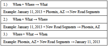
Space and time are both continuous. This presents a challenge for GIS due to the nature of computer systems and databases[51, 43]. Regardless, for purposes of objective measurement observations of the phenomena or object must be broken down into discrete units. When selecting units, it has been found that resolution and scale must be considered [43, 52].

Discretization of phenomena are similar in some aspects with space and time yet there are some important differences. Spatially, limitations for GIS are organized in raster, vector or an extension of one of these[53]. Euclidian logic, in most cases, provides discrete grid cells or the necessary coordinate locations for features such as points, lines and polygons. Time, must also be subdivided into units. These units are often referred to as events along a continuum. What is unique about time is that it is one directional, so the idea of an absolute timeline with stored events is a viable means for storing temporal information as they relate to objects stored in GIS[54, 43]. In addition, the topological variability for time is greater with a much wider array of possible scenarios [43].

If successful storage of space and time data can be accomplished the next area of active development deals with concepts of movement or patterns.[55, 45, 43]. Classifying patterns in both space and time is an important part of understanding complex phenomena, this includes the understanding of GIS networks. Consideration of temporal changes in network patterns over time in terms of not only spatial patterns, but temporal patterns would be an added benefit to GIS network analysis. The following table shows the various behaviors of objects or phenomena both spatially and temporally.

Table 3. Spatial/Temporal Patterns[43]

In direct support of GIS network pattern categorization, “Space and time have a framing role and consequently spatial-temporal representation is important for developing explanations”[49]. Methods in using map symbology, “snap shots” or time slices, oscillating colors, supplemental graphs, Virtual Geographic Environments, and animations are all notable examples of how various patterns within a GIS network could be represented successfully[43, 50].

A fundamental goal for space-time GIS is the idea of moving forward from “World History Models to Process Models”[43]. In other words, a deliberate part of a space-time GIS is the iterative cycle of taking “Location and Time” based representations, working through “Object-based” representations to allow for the production of new knowledge. In 2008, Peuquet added the “why” and “how” to the top of her original Triad to further this point.

What was not found in the literature reviewed were real world example how these concepts could be applied to road network analysis. Although a considerable amount of data and research has been applied to the subject, dealing with concepts in terms of what, when and where in GIS is still needed.

3. Research

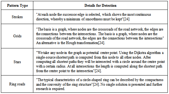
Research considerations conducted by others to date have focused patterns in GIS networks. Patterns of interest include grids, ring roads, stars, and strokes as discussed by Marshall [20]. The patterns identified by Marshall have been explored through various systematic approaches to automatically have computers isolate them. These studies have been done for each pattern type in a deductive fashion. Inductive analysis based on a metric or index for repeatedly identifying these patterns is an ambitious objective. Serving as a common denominator for comparing patterns the proposed method will also look at non-spatial metrics for comparison. Additionally, a review of the detected patterns in the networks and how they change over time is an added goal. Further, this study will test the DAS method against a cognitive pattern identification survey. Ideally, this will provide new knowledge in computer and human pattern recognition. The knowledge gained in this study will determine if a new pattern detection method based on Density, Angles, and Shape can successfully isolate various patterns. Development and testing of a new method for network pattern detection expands to include these questions in depth:

1.) Using simulated grid, ring road, star, and stroke patterns, can a single GIS tool provide the ability to identify these patterns reliably and repeatedly? Further, what additional patterns are detected within the targeted networks?

2.) Present a study to consider geographic areas where patterns in the 2010 road centerlines and 2000 road centerline networks.

3.) Present an approach for participants to identify the most prominent patterns in a series of maps showing networks, can a GIS tool identify these same patterns and quantitatively provide comparative results.

3.1. The DAS Method

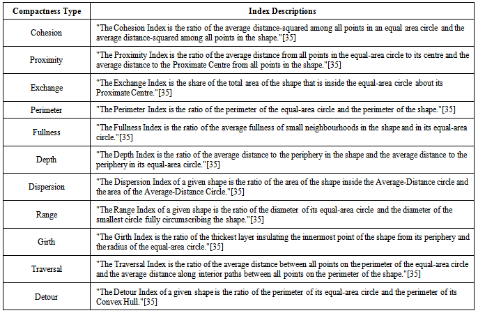
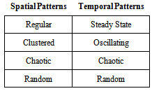
DAS is a GIS model that requires a network in GIS. DAS stands for the variables of features that will be used to derive a single quantitative metric for pattern detection. D, stands for density, and will measure the density of nodes within the target geographic dataset. A, stands for angles, and will measure the edge angle for features. S, stands for shape and will be a calculated value for polygons that are inherent with networks for areas enclosed by the edges. Further description of each variable in DAS are described below:

• Density, provides how compact the location of nodes within a network. This value will be calculated for road networks using a constrained method on the network. The density measures will reside with the nodes and persist as a value from 0 to 1, where 0 is least dense and 1 is very dense.

• Angles, show how the edges are oriented using angles in degrees. These values will reside with the edges and show a bearing. Values will range from 0 to 359 in the form of degrees.

• Shape, will use the property of cohesiveness or compactness of polygons. In the form of an index value, the compactness score for polygons in the DAS method will range from 0 to 1. 0 will be least compact shape, while a score of 1 would be the form of a perfect circle (A circle is the most compact or cohesive shape).

The baseline target patterns DAS will be calibrated with include grids, stars, circles, and strokes. Grids are regular rectangle patterns. Stars are patters that radiate from a central location. Circles or by-pass patterns typically encircle an area. Finally, strokes are longer segments where other edges feed. Strokes are sometimes described as a main road in a city. Real examples of each of these patterns are pictorially shown here:

Figure 3. Target Patterns Examples: A) Grid Pattern, B) Start Pattern, C) Circle, D) Strokes

Network's in GIS are vector datasets comprised of nodes and edges. For example, in road networks, the nodes represent intersections and the edges represent road centerlines. In a stream, the nodes could be where a tributary meets a larger section of a river. The rivers and streams would be represented by edges. These features, in this special format will be used as a starting framework for the DAS method. Additionally, polygons will topologically be added to represent areas enclosed by edges and are also incorporated into DAS.

Map scale and projection will need to be constrained for these studies. This is important because the DAS method will rely on Euclidean shape and direction variables. Although the model is capable of running at virtually any scale, the review and analysis will take place within a range of 1:50,000 to 1:100,000. At this scale, map distortion will be limited. To ensure this, an equal-area and conformal projection will be tested to ensure calculated results do not significantly impact results

The DAS method and following studies will use US Tiger Census road centerline files. Limitations in US Census Tiger data will predetermine the spatial accuracy and level of generalization for source data and have will have some impact on the output results of these studies. Due to the wide coverage and the temporal availability of road network geometry these shortcomings will be accepted. Future testing of the pattern identification with the DAS method would be improved with a localized map projection and road network geometry that is more up to date and has authoritative absolute spatial and temporal accuracies that go beyond the requirements of the US Census data. Regardless, the testing of the DAS method will not be limited in terms of testing the viability of DAS with US Census road centerline data.

3.2. Technology Stack

The DAS model should be implemented using commercial software developed by Environmental Systems Research Institute, Inc. (Esri). The version of software to be used will be 10.2. The DAS model will perform against a Geodatabase. A Geodatabase is a format for storing geographic features and data specifically created by Esri. More specifically, a network Geodatabase will be used as a starting point for managing the nodes and edges of road networks for my case study areas. Polygons will added to the Geodatabase to help identify the shapes of areas enclosed by roads. A final layer of information will be included within the Geodatabase representing patterns and DAS method metrics.

3.3. Solving DAS

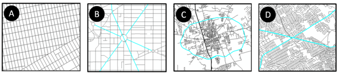
DAS should primarily be tested using three variables, density, angles and shape. Density calculation will be carried out in the Spatial Analyst Extension of ArcGIS. Consideration and testing will need to be conducted for an intersection density approach that best fits the objectives for the DAS method. Options include point density, kernel density and others. To ensure density measures are working at the scale common to road intersections for the targeted patterns. For example, if a density metric that covers too much area is used then density patterns may not be contained in results. Therefore, the density index would not be of use for pattern identification within networks. Based on the same foundation completed in Borruso's development of a Network Density Estimation[56]. The Kernel Density Estimation (KDE) will be performed.

(1)

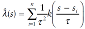
where λ(s) is the estimate of the density of the spatial point pattern measured at location s, s_i the observed i^th event, κrepresents the kernel weighting function and is the bandwidth"[56].

For each density measure option, a raster surface with a classification score for each cell will be produced. The class value from the raster surface will then be spatially applied back to the intersection point as an attribute. This will be done so that each node will be attributed with its own density.

Angles are the second DAS metric required for the calibration of the DAS method. Angles will be computed based on the azimuth of each line using the end points. The resulting values will range between 0 to 360 degrees. Calculating the angles will be completed with the following approach:

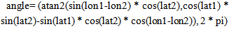
(2)

where the input of coordinates for each line segment will require a latitude (lat1,2) and longitude (lon1,2).

An example of how this looks when a sample network is labeled with the calculated angles is show in the following figure:

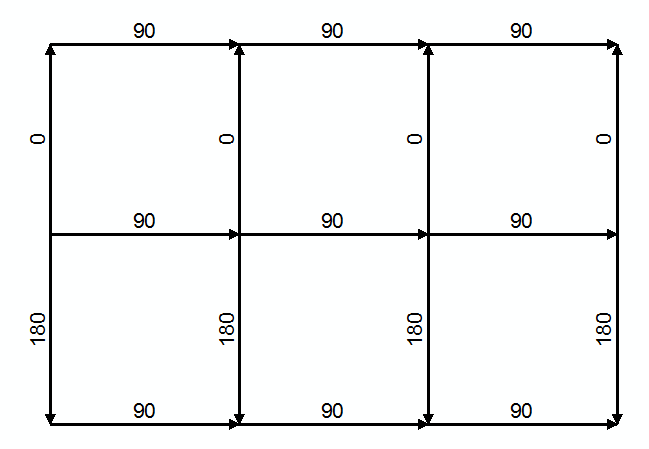
Figure 4. A network showing with edge angles labeled

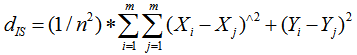
Features that have a "flip in direction" at the crossing of an intersection may be a challenge. In the example just shown, the interior edges have directions that point outward from the midline intersections. This may require the identification of symmetry or isolation of angles where polar opposite directions are matched and assimilated into a continuation for one of the presiding edge angles. For example, if one feature has an angle of 180 degrees and after an intersection the angle is 0 degrees, the value of 180 degrees would need to be applied to both segments for proper modeling.

The third variable that will be used within the DAS model will be that of shape. This will be done by using the topology of the network where edges enclose polygons. Each shape's cohesiveness will be calculated based on a formula by Angel et al.[35] that provides the Cohesion Index. For this calculation, an index value of 1 would be in the form of a circle. The logic for finding the Cohesive Index by Angel is as follows:

(3)

"Calculate the average inter-point distance square d_IS between a sample of m random points in the shape.

Patterns were digitized in a "perfect form" from scratch. "Perfect form", in this case means that intersection spacing, angles of the roads and the shapes contained within polygons enclosed by the edge features will be synthetic, symmetric and spaced in an ideal fashion. These patterns will be completed at a scale of 1:50,000 using a map projection that offers the lowest possible distortion of shape, area and direction. For the overall study, this will provide the necessary calibration. This is crucial because a baseline will allow processing against areas that are not ideal. This is important because it offers the opportunity to ask the question, how far statistically from "ideal" are other observed areas or patterns?

Limits of this study are bound to geographic features and apply primarily to road features at appropriate scales. By running the DAS method on ideal conditions, it is anticipated that there shall be issues within the real world that the model may not identify. These limits were considered for the development of the pilot study.

3.4. Pilot Study

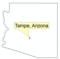
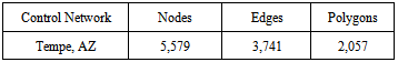
The simulated patterns created will be done in Euclidean space. The key importance is that each pattern will be mapped for analysis. To further check the validity of the calibration Tempe, Arizona will be included within this study. The use of a "real" city is deliberate to sample the methods of analysis against patterns that are not in the "perfect form" Additionally, through subjective observation, Tempe, Arizona offers stroke and grid patterns detectable without a GIS analysis. The following network datasets will be used to test the DAS method:

1. Tempe, Arizona

2. Grid Pattern Simulation

3. Star Pattern Simulation

4. Ring Pattern Simulation

5. Stroke Pattern Simulation

6. Branch/Tree Pattern Simulation

As an example, the input will be quantified in terms of its geographic composition based on the number of features. This will be important in terms of statistical significance when comparing larger network datasets. The following table shows the feature counts for Tempe, Arizona.

Table 4. Example of network description in terms of elements

These patterns will be constructed by placing features at precise spacing and angles. For example, intersections will be placed at exactly quarter mile spacing with 90 degree angles. Network topology will be added and polygons will be created. For the City of Tempe, Arizona, US Census road centerlines will be obtained and converted into a network model. Polygons will also be created for areas contained within the road line work.

The index scores for each pattern will be the results of the DAS calculations. I envision these scores will be used as algorithms that will be run with a final GIS tool using the Python scripting language. The resulting index range values. These range values will be in the form of a mean score along with standard deviations. Essentially, for each simulated pattern type a "normal" index value with +/- standard deviations.

Nodes, edges, and polygons will have a corresponding metric value. Either through a relational feature class or an independent feature class, lines will be created based on the metrics of the underlying features (Nodes, edges, and polygons). This will present a final metric to represent each pattern. For example, the grid pattern will have a density score, angle score, and shape score for the pattern. This will then be the index that can be used later to identify patterns. The results will be loaded into a polyline feature class based on the original line work geometry.

For Tempe, Arizona, the final scores offer insight into how random or mixed scores are compiled. The City of Tempe also provided an initial test to determine how different aspects of the DAS method perform individually and collectively. For example, individually, a shape compactness index was used to analyze the City of Tempe, Arizona. A thematic map shows a standard deviation classification of compactness index scores. Clearly there is a tendency for the less compact polygons to represent road features that would resemble strokes. Isolating statistical mean values and testing confidence intervals used to test each of the index populations. Margin of error, uses the standard deviation, sample sizes, and the level of confidence. Further modeling of the results in scatter plots show the results for each pattern type.

Where polygons were derived by closed areas within the road network. The thematic map is classified by standard deviations with the assumption of normal distribution. The linear features shown in dark shades are representative of polygons with low cohesion, or compact index scores, and these show stroke pattern tendencies.

Normality testing on each of the DAS variables (Density, Angles, and Shape) must be further tested against another variable defined as having a normal distribution. As an example, a Kolmogorov-Smirnov One-Sample Test will should be conducted to determine how DAS is performing statistically. The intention would be to assess and ensure the results are valid and ready for use in study two and study three.

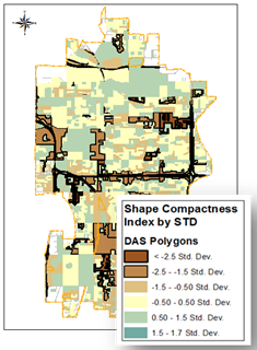
Figure 5. Analysis Results for Tempe, Arizona

This study has been deliberately designed to provide an overall support of internal validity. Pattern identification conducted on non-simulated patterns in later studies will depend on the results from this pilot. This case study therefore not only helps to calibrate the DAS approach, but also helps to ensure ideal conditions are realized, before applying the DAS method to real world network investigations.

Using a simulated grid, ring road, star, stroke, and branched pattern the implementation of the DAS method will be tested to provide the ability to identify these patterns. By having a non-synthetic network model used (Tempe, Arizona), anomalies and challenges for implementation will be acknowledged and addressed within this first study. The City of Tempe, Arizona and the synthetic road network will be tested with DAS to determine the following objectives through the corresponding methods of comparison:

Table 5. Showing criteria and methods

3.5. Large Urban Analysis

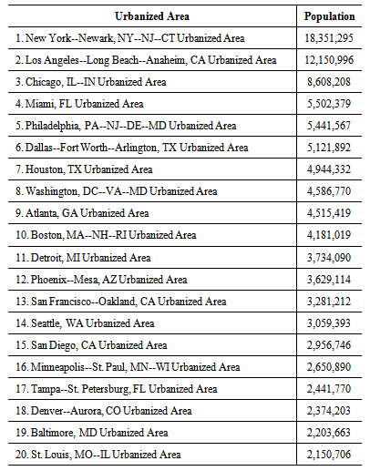
To broaden the geographic scope as well as the temporal scope for the DAS model this further study put the method to the test. Locations for this case study will be the top twenty most populated 2010 Urbanized Areas found in the United States. These areas have been selected due to their large populations and the likely high quantity of road network patterns. Temporally, the DAS model will be run on the 2010 road network as well as the 2000 road network within areas delineated by the 2010 Urbanized Area Boundaries. This will provide two snapshots in time for comparative analysis. In the April 2010 US Census there were 3,592 polygons representing Urbanized Areas. These were Urbanized Areas that had a population over 50,000. 3,535 of these Urbanized Areas were located in the continental United States. The top twenty most populous will be sub selected for this case study. This selection was represents over 100 million inhabitants and 40% of the population in the United States living in Urbanized Areas. A better understanding of road network patterns (meaning more than looking at just grids or a single point in time) serves to provide new knowledge about the following Urbanized Areas and their populations as shown in the following table:

Table 6. Top twenty most populous Urbanized Areas (US Census Bureau - release date April, 2012)

Geographically this study should encompass the following major cities where the 2010 most populous Urbanized Areas are situated:

Figure 6. Cities within the top twenty most populous Urbanized Areas in the United States (US Census Bureau - release date April, 2012)

3.6. Required Data and Acquisition

The data required for this study is US Census Bureau information. Decennial products will serve as a secondary source for the application of the DAS method. The US Census includes a comprehensive road centerline file by county. This data has been acquired by FTP and has been merged into road network datasets for each Urbanized Area. To ensure each Urbanized Area is fully represented a buffer of ten miles around each of the Urbanized Area was created and road centerline files were incorporated. The reason for this is to allow the DAS model to be run on the outer edges of the Urbanized Areas where Urban Geographers may gain new insight into land settlement. This is also where the comparison of the 2000 US Census road network and the 2010 US Census road network is anticipated to show space-time analysis contributions. Typical land-use or urban growth analysis is are done with remote sensing techniques or using population demographics as was conducted by Brown[190]. Alternatively, this study will provide a first GIS network based change detection method for space-time output.

Road names, address ranges and road direction will not play a role in the application of DAS. Further, directional turn tables will not be required for the DAS method. Polygons, that contain road segments that do not complete the topology for enclosing an area, such as a cul-de-sac will be addressed by the tool when indexing angles for road segments and will not be included with the shape compactness index portion of the automatic processing. This is anticipated to not be an issue as these segments of road will not be important for the identification of target patterns (grid, star, ring road, and strokes).

3.7. Analysis Approach

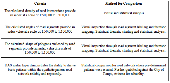
The data shall be analyzed by running the DAS model against each Urbanized Area road network. As the dependent variables, each urbanized area will have a number of statistical results compiled within a final DAS Polyline. The process will mirror the process conducted in the first case study, however, this will be done over a much larger area and with many more features.

Three levels of investigation are anticipated. One, a visual inspection will be conducted by using thematic mapping techniques. Due to the quantitative quality of the DAS method, density, angles, and shape will be readily available for Equal Interval, Quantile, Natural Breaks, and by Standard Deviation classification methods. A second approach will be to review the DAS model results by considering a cluster score. In order to isolate certain patterns, scores will be isolated on the edges where patterns are identified. These will also be visually inspected specifically for locations where patterns are known to exist. This will take advantage of the first study's results where regular patterns were scored and will provide a likelihood score for a pattern match. Finally, the road network results will be statistically analyzed. Plotting the results of each Urbanized Area or the dependent variable against the synthetic road network or independent variable it is anticipated that the quantity of the different pattern types will be presented. This will include measures of statistical significance. Another analysis that should be carried out will be the comparison of results for 2000 and 2010 road network pattern scores from the DAS method. These results will be considered in terms of space-time pattern where results could show a regular, clustered, random or chaotic outcome. The effectiveness of this study and versatility of the DAS model will be done through statistical means. Based on the first case study, DAS metrics will serve as the baseline for "perfect scores". The study will then look at areas where a statistical relationship is present.

To analyze the resulting patterns in the datasets once the DAS model is run will require statistical analysis where the dependent and independent variables will be analyzed and plotted. A comparison of the results will be conducted for a sample against the grid patterns. Additionally, alpha, gamma, and GTP analysis will be carried out for the same sample data to further test the DAS method. This will require a statistical software for analysis. As with the analysis of Tempe, Arizona, the DAS index values will reside on a polyline GIS layer. The scores will include a likelihood score for grid, star, ring road, and stroke patterns. For the processed areas, the DAS GIS method should identify road network patterns for 2010 road centerlines and 2000 road centerline in locations where change is likely to have occurred.

3.8. Human Cognition

Another important aspect to evaluating computational pattern recognition, overlooked by many is how the computer method measures up to human analysis. A survey where participants identify the most prominent patterns in a series of maps showing road networks offer a way to check this. The objective would be to see if the DAS method quantifiably identifies patterns competitively. This means survey participants would identify a prominent pattern within a map that shows only road line work. DAS will then be run on the same geographic area. The study area locations will each be areas found in the top ten US Census most populous Urbanized Areas. The data required for this case study will already be available and analyzed.

An exploratory survey with a small sample of three colleagues was conducted to assist with development and to provide a baseline for practicality. It was decided that each colleague would provide very basic information such as gender, age and the number of locations they had resided in their lifetime. Important to anonymity, each participant in an actual survey will be given an identification number that will be indexed to their name and kept in confidentiality. The reason for these questions was to ensure I would be able to identify the ten maps within their survey and could gauge qualitatively how comfortable they may be with looking at maps of locations they have never seen before. The assumption would be that individuals who had only lived in a single location may view a new map differently then someone who has moved about in their lifetime.

Ten map plates were created at scales that range from 1:50,000 to 1:100,000 where census road network centerlines were the only features displayed on the maps. The area represented in each map template cover areas found within the top ten most populated urbanized areas. The road centerline files used are from the 2010 US census. Figure 7 shows samples of some of the basic map templates used in the test survey.

The instructions requested that each participant highlight the "Most Prominent" pattern they see. No other instructions or prompting was provided. The results will then be compared to the same map location with the DAS method.

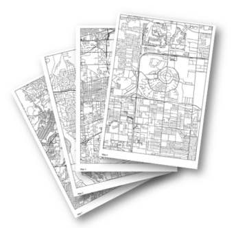
Figure 7. Sample map plates for survey instrument

Each participant highlighted different areas for most maps when compared across the results. Some identified grid patterns, while others honed in on stokes or ring roads. The goal of the study was to see if the patterns identified by participants are also the most prominent when compared to results derived by the DAS method. In this case study, the DAS method, still in development will need to be applied to each of the same areas that were evaluated by the participants, with a larger population sampling. Statistically, through the index and output polyline feature class of the DAS method, a prominent pattern will be identified. This will allow for a more in depth comparison of the surveyed results and the DAS method where the survey results will act as the dependent variable in a spatial and statistical analysis. For proper spatial alignment, each map from the surveys were scanned, registered, rectified and digitized so spatial representation of the highlighted pattern locations will be spatial-statistically scrutinized for each map by each participant.

4. Results, Significance and Future Studies

The significance of this research contributes to our body of knowledge in three ways. The first contribution is methodological. The implementation and testing of the DAS method, although an early concept, will be the first to test for pattern identification in networks using only spatial metrics for use in the GIS toolkit. Second, the DAS will provide analytical results for a number of locations using two distinct times. This will provide the inauguration of network pattern analysis that generates results worthy of future research for cause and effect based studies. Third, the research presented here will further explore cognitive aspects to human map interpretation when focusing on spatial network patterns.

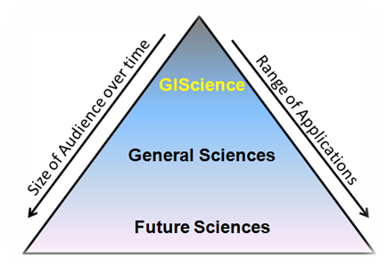
Figure 8. Research beneficiaries

Three audiences will benefit from this research. GIScientists, scientists, and future scientists will be provided a direction to push for a series of quantitative results derived by DAS as well that has been tested against other strategies. In GIScience, new strategies for pattern identification in network datasets independent of the network type or pattern will help advance efforts in network analysis, spatial analysis and mapping of linear features.

The larger audience that benefits from this research are the general sciences. By design, the DAS method produces new information about spatial patterns in networks. This information should be further analyzed to assess cause and effect relationships surrounding networks. In other words, the patterns and quantitative representation of networks in the hands of social scientists, biologists, hydrologists, environmentalists, general practitioners and subject matter experts will provide a new set of knowledge. The importance to each beneficiary will depend on whether their research problems are spatially bound and a network model is appropriate.

The third audience this project will serve reaches into the future where a positivist perspective on technology would envision a self-thinking system. Identification of patterns with the DAS method, is methodical in its present state, and will require a great deal of human interaction for operation. Looking into the future, an enhanced DAS method could be a building block for future scientists to automate spatial pattern recognition. Further, such a system that then would teach itself to better interpret network patterns would be logical. Autonomous vehicles, aircraft navigation, self optimizing control systems, are examples. Future science, the DAS method, and artificially intelligent could pose significant changes in how we look at spatially related problems in society and out environment. A closer look could provide critical knowledge for decision making on such important themes as our environment, society, and other complex systems that sustain life on Earth.

ACKNOWLEDGEMENTS

The author thanks members of Data Transfer Solutions, LLC for support. Special thanks to Professor Robert Balling Jr. of Arizona State University and Professor Christopher Lukinbeal of University of Arizona for moral support and encouragement.

References

[1]  Curtin, K.M. 2008. "Linear Referencing". The Encyclopedia of Geographic Information Science, 261-264. Karen Kemp ed. Sage Publications.
[2]  Ficsher, Manfred. 2003. GIS and Network Analysis. Handbook 5 Transport Geography and Spatial Systems. Hensher D. Button K. and Stopher P. eds.
[3]  Mackaness, W., Edwards, G. 2002. The Importance of Modeling Pattern and Structure in Automated Map Generalization. Joint Workshop on Multi-Scale Representations of Spatial Data, Ottawa, Canada.
[4]  Zhang, Q. 2004. Modeling Structure and Patterns in Road Network Generalization. ICA Workshop on Generalization and Multiple Representations, Leicester, United Kingdom.
[5]  Gastner, Michael T., Newman, M. E. J. 2004. The Spatial Structure of Networks. Statistical Mechanics. Eur. Phys. 49, 247-252.
[6]  Newman, Mark EJ. 2003. The Structure and function of complex networks. SIAM Review. Vol. 45:2. pp. 167-256.
[7]  Wantanabe, Daisuke. 2010. A Study on Analyzing the Grid Road Network: Patterns using Relative Neighborhood Graph. The Ninth International Symposium on Operations Research and Its Applications (ISORA'10). Chengdu-Jiuzhaigou, China, ORSC & APORC. pp. 112-119.
[8]  Usui, Hiroyuki, and Asami, Yasushi. 2011. An Evaluation of Road Network patterns based on the Criteria for Fire-Fighting. Cybergeo: European Journal of Geography.
[9]  Jiang, B. and Claramunt, C. 2004. A Structural Approach to Model Generalization of an Urban Street Network. GeoInformatica. Vol. 8:2. pp. 157-171.
[10]  Yang, Bisheng, Luan, Xuechen, Li Qingquan. 2010. An adaptive method for identifying the spatial patterns in road networks. Computers, Environment and Urban Systems. Vol. 34. pp. 40-48.
[11]  Albers, Heidi J. Ando, Amy, Bu, Meidan, Wing, Michael G. 2012. Road-network agglomeration, road density, and protected-area fragmentation. Letters in Spatial and Resource Sciences. DOI 10.1007/s12076-012-0078-z.120.
[12]  Touya, Guillaume. 2010. A Road Network Selection Process based on Data Enrichment and Structure Detection. Transactions in GIS. Vol. 14:5. pp. 595-614.
[13]  Xie, Feng and Levinson, David. 2006. Measuring the Structure of Road Networks. Geographical Analysis.
[14]  Pengyao, YE, Hong, Yang. 2011. Concentration Degree Analysis of Stroke-based Urban Road Network Topology. ICTE 2011, ASCE 2011. pp. 511-516.
[15]  Heinzle, Frauke, Anders, Karl-Heinrich, Sester, Monika. 2006. Pattern Recognition in Road Networks on the Example of Circular Road Detection. Geographic Information Science. pp. 153-167.
[16]  Gastner, Michael T., Newman, M. E. J. 2004. The Spatial Structure of Networks. Statistical Mechanics. Eur. Phys. 49, 247-252.
[17]  Ficsher, Manfred. 2003. GIS and Network Analysis. Handbook 5 Transport Geography and Spatial Systems. Hensher D. Button K. and Stopher P. eds.
[18]  Curtin, Kevin. 2007. Network Analysis in Geographic Information Science: Review, Assessment, and Projections. Cartography and Geographic Information Science. 34(2). 103-111.
[19]  Duo, N. 2004. Graph Theory with Applications to Engineering and Computer Science. PHI Learning Pvt. Ltd.
[20]  Marshall, Stephen. 2005. Streets and Patterns. Spon Press. Taylor & Francis Group, New York.
[21]  Takhteyev, Yuri, Gruzd, Anatoliy, Wellma, Barry. 2012. Geography of Twitter Networks. Social Networks. Vol. 34. pp. 73-81.
[22]  Heinzle, F., Anders, K.H., and Sester, M. 2005. Graph based approaches for recognition of patterns and implicit information in road networks. Proceedings of the 22nd International Cartographic Conference. pp. 11-16.
[23]  Diakoulaki, D., Mavrotas, G., and Papayannkis. 1995. Determining objective weights in multiple criteria problems: the critic method. Computers & Operations Research. Vol. 22:7. pp. 763-770.
[24]  Heinzle, F. Anders, Sester M., 2007. Automatic Detection of Patterns in Road Networks - Methods and Evaluations. Proceedings of Joint Workshop Visualization and Exploration of Geospatial Data, Stuttgart. Vol. 36.
[25]  Boyce, Ronald R., Clark, W. A. V., 1964. The Concept of Shape in Geography. Geographical Review. 54(4): 561-572.
[26]  Wentz, Elizabeth. 2000. A Shape Definition for Geographic Applications Based on Edge, Elongation, and Perforation. Geographical Analysis. 32(1): 95-112.
[27]  Metaxas, Dimitris, Terzopoulos, Demetri. 1993. Shape and Nonrigid Motion Estimation through Physics-based Synthesis. Pattern Analysis and Machine Intelligence. IEEE Transactions on, 15:6, pp. 580-591.
[28]  Chazal, P, Flynn J., Reilly R.B. 2005. Automated processing of shoeprint images based on the Fourier transform for use in forensic science. Pattern Analysis and Machine Intelligence, IEEE Transactions on. 27(3): pp.341-350.
[29]  Brown, Daniel, Johnson, Kenneth, Loveland, Thomas, Theobald, David, 2005. Rural Land-Use Trends in the Conterminous United States, 1950-2000. Ecological Applications, 15(6): 1851-1863.
[30]  Pizer, Sephen M., Burbeck, Christina A., Coggins, James M., Fritsch, Daniel S., Morse, Bryan S. 1992. Object Shape before Boundary Shape: Scale-space Medial Axes. Journal of Mathematical Imaging and Vision. Vol. 4:3, 303-313.
[31]  Belongie, S., Malik, J., Puzicha, J. 2002. Shape matching and object recognition using shape contexts. Pattern Analysis and Machine Intelligence, IEEE Transactions. Vol. 24:4. pp. 509-522.
[32]  Klippel, Alexander, Hardisty, Frank, Li, Rui. 2011. Interpreting spatial Patterns: An Inquiry Into Formal and Cognitive Aspects of Tobler's First Law of Geography. Annals of the Association of American Geographers. Vol. 101:5. pp. 1011-1031.
[33]  Sanders, Ralph A., Porter, Philip W. 1974. Shape in Revealed Mental Maps. Annals of the Association of American Geographers. Vol. 64:2 pp. 258-267.
[34]  Montello, Daniel R. 2002. Cognitive Map-Design Research in the Twentieth Century: Theoretical and Empirical Approaches. Cartography and Geographic Information Science. Vol. 29:3, pp. 283-304.
[35]  Angel, S., J. Parent, et al. 2010. Ten compactness properties of circles: measuring shape in geography. Canadian Geographer 54(4): 441-461.
[36]  MacEachren, A.M. 1985. Compactness of Geographic Shape: comparison and evaluation of measures. Geografisca Annaler, Series B, 67(1): 53-67.
[37]  Lee, David R., Sallee, Thomas. 1970. A Method of Measuring Shape. Geographical Review. 60(4): 555-563.
[38]  Bunge, William. 1962. Theoretical Geography. C.W.K. Gleerup, Publishers/Lund. The Royal University of Lund, Sweden.
[39]  Atwood, Emily. 2004. The TOSS Method: An Enhanced Polygon Pattern Analysis Method for Nominal Data. Master’s Thesis. Arizona State University.
[40]  Wentz, Elizabeth. 1997. Shape Analysis in GIS. Proceedings of AUTO-CARTO. 204-213.
[41]  Atwood, Emily, Wentz, Elizabeth A. 2008. Pattern Analysis Based on Type, Orientation, Size, and Shape. Geographical Analysis. 40(2): 97-122.
[42]  Newman, Mark EJ. 2006. Modularity and community structure in networks. Proceedings of the National Academy of Sciences. 103(23). pp. 8577-8582.
[43]  Peuquet, Donna, 1994. It’s about Time: A conceptual Framework for the Representation of Temporal Dynamics in Geographic Information Systems. Association of Annuls of the Association of American Geographers. Vol. 84. No. 3. 441-461.
[44]  Miller, Harvey J. 2005. A Measurement Theory for Time Geography. Geographical Analysis Vol. 37. pp. 17-45.
[45]  Fisher, PF. 2005. Re-presenting GIS. John Wiley & Sons, LLC.
[46]  Kwan, Mei-Po, and Jiyeong Lee. "Geovisualization of human activity patterns using 3D GIS: a time-geographic approach." Spatially Integrated Social Science 27 (2004).
[47]  Langran, Gail, Chrisman, Nicholas. 1998. A Framework for Temporal Geographic Information. Cartographica, Vol. 25, No. 3, 1-14.
[48]  Massey, Doreen. 1999. Space-Time ‘Science’ and the Relationship Between Physical Geography and Human Geography. Vol. 24, No. 3, 261-276.
[49]  Raper, Jonathan, Livingstone, David. 2001. Let’s get real: spatio-temporal identity and geographic entities. Transactions of the Institute of British Geographers, Vol. 26 No. 2. pp. 237-242.
[50]  Peuquet, Donna, 2008. The Multi-Representation of Space-Time Information. Key Note Address. Virtual Geographic Environment Hong Kong University. Jan. 7.
[51]  Couclelis, H. 2009. Rethinking time Geography in the Information Age. Environment and Planning. A, 41:7. 1556.
[52]  Peuquet, Donna J. 2002. Representations of Space and Time. The Guilford Press.
[53]  Peuquet, Donna J., Duan, Niu. 1995. An Event-Based Spatiotemporal Data Model (ESTDM) for Temporal Analysis of Geographical Data. International Journal of Geographical Information Systems. Vol. 9:1, pp. 7-24.
[54]  Anderson, Sharolyn. 2002. Design and Implementation of Spatio-Temporal Interpolation Model. Ph.D. Thesis. Arizona State University.
[55]  Dodge, Somayeh, Weibel, Robert and Lautenschüz, Anna-Katharina. 2008. Towards a Taxonomy of Movement Patterns. Information Visualization. Vol. 7:3-4. pp. 240-252.
[56]  Borruso, Giuseppe. 2008. Network Density Estimation: A GIS Approach for Analyzing Point Patterns in a network Space. transactions in GIS. 12(3): 377- 402.
[57]  Brown, Daniel, Johnson, Kenneth, Loveland, Thomas, Theobald, David, 2005. Rural Land-Use Trends in the Conterminous United States, 1950-2000. Ecological Applications, 15(6): 1851-1863.