Opaluwa Y. D, Adejare Q. A, Suleyman Z. A. T, Abazu I. C, Adewale T. O, Odesanmi A. O, Okorocha V. C
Department of Surveying & Geoinformatics, Federal University of Technology, Minna, Niger State, Nigeria
Correspondence to: Adejare Q. A, Department of Surveying & Geoinformatics, Federal University of Technology, Minna, Niger State, Nigeria.
| Email: |  |
Copyright © 2012 Scientific & Academic Publishing. All Rights Reserved.
Abstract
The atmosphere causing the delay in GPS signals consists of two main layers, ionosphere and troposphere. The ionospheric bias can be mitigated using dual frequency receivers. Unlike the ionospheric bias, the tropospheric bias cannot be removed using the same procedure. Compensation for the tropospheric bias is often carried out using a standard tropospheric model. In order to investigate the impact of different dry tropospheric models on GPS accuracy, simultaneous hourly observations was carried out at some selected stations in Minna. The tropospheric errors obtained using five standard tropospheric models namely, the Saastamoinen model (which was adopted as the standard model), Hopfield model, Davis et al. model, Saastamoinen model (Using Ground Meteorological Data) and Altshuler and Kalaghan model were compared. It was deduced from the results that at all the stations, the Saastamoinen Model (Using Ground Meteorological Data), has 100% correlation with the adopted standard Dry Tropospheric Model (Saastamoinen model). While a standard error of 0.285mm, 1.446mm and 2.899mm were respectively obtained for Davis et al. Model, Hopefield model and Altshuler and Kalaghan (A&K) Model. However, the statistical test performed on the overall results indicated that there is no significant difference in the performance of the five tropospheric models at 0.05 significance level. It was therefore, concluded that either of the five models evaluated in this study can perform well in the study area, nevertheless, the choice of Saastamoinen Model, Saastamoinen Model (Ground Meteorological Data) and Davis et al. Model will be more preferable.
Keywords:
Ionospheric Bias, Troposheric Bias, GPS Signal, Tropospheric Models
Cite this paper: Opaluwa Y. D, Adejare Q. A, Suleyman Z. A. T, Abazu I. C, Adewale T. O, Odesanmi A. O, Okorocha V. C, Comparative Analysis of Five Standard Dry Tropospheric Delay Models for Estimation of Dry Tropospheric Delay in Gnss Positioning, American Journal of Geographic Information System, Vol. 2 No. 4, 2013, pp. 121-131. doi: 10.5923/j.ajgis.20130204.05.
1. Introduction
1.1. Background to Study
The propagation delay induced by the electrically neutral atmosphere, commonly known as the tropospheric delay, is one of the most difficult-to-model errors affecting space geodetic techniques. An unmodelled tropospheric delay affects mainly the height component of position and therefore constitutes a matter of concern in space-geodesy applications, such as sea-level monitoring, post-glacial rebound measurement, earthquake-hazard mitigation, and tectonic-plate-margin deformation studies, where the highest possible position accuracy is sought, hence the improvement in tropospheric delay modelling is therefore essential[19].When travelling through the electrically-neutral atmosphere, radio signals used by radiometric techniques are affected by the variability of the refractive index, causing an excess path delay and ray bending. The effect is commonly known as tropospheric propagation delay (or simply tropospheric delay), even though this designation is misleading, as the stratosphere has a significant contribution to the total delay [8]. The troposphere is an effectively non-dispersive region up to frequencies of approximately 15GHz for microwave signals. In other words the propagation through the troposphere is not frequency dependent.The delay caused by the troposphere can be separated into two main components: the hydrostatic delay and the wet delay [13]. The zenith hydrostatic delay (dry component) contributes about 90% of the total delay to the tropospheric delay[16]. The dry component is determined with high accuracy by many tropospheric delay models derived from surface measurements. Since the dry part of the troposphere is in hydrostatic equilibrium, the ideal gas law can easily be applied to it. The wet component, however, is difficult to predict because of the irregular distribution of liquid water and water vapour both horizontally and vertically in the troposphere. Although the wet component of the delay constitutes less than 10% of the total effect[9], it still causes the limiting uncertainty in determining a very accurate remedy for the total delay. The tropospheric delay is difficult to fully correct and constitutes one of the major residual error sources in modern space geodetic techniques such as–DORIS (Doppler Orbitography and Radio-positioning Integrated by Satellite), GPS (Global Positioning System) and VLBI (Very Long Baseline Interferometry) – affecting mainly the estimates of the height component of position[16].
1.2. Statement of Problem
Tropospheric delay is one of the major errors in Global Navigation Satellite System (GNSS) Positioning. Several models exist for estimating the magnitude of this error in the determined positions, but the level of refinement attainable with each of the models differs. Furthermore, the effect of tropospheric delay has been accounted for in dual frequency GPS receivers, but the impact is still significant in single frequency receivers. Since most GNSS users in the study area cannot easily afford dual frequency receiver, there is the need to assess the performance of some standard tropospheric models in the area. Therefore, this research seeks to compare some dry tropospheric delay models in Minna using data observed with single frequency Differential GPS (DGPS).
1.3. Aim and Objectives
The aim of this research is to identify the optimum dry tropospheric model using single frequency GPS receivers. Therefore, the objectives that will assist in achieving the above aim include the following:- To carry out DGPS observations at three (3) epochs of the day (i.e. morning, afternoon and evening), as well as atmospheric parameters such as temperature, relative humidity, pressure, etc at some selected stations in Minna.- To estimate the amount of dry tropospheric delay with each model at various epochs of observation using a program written in Java programming language.- To examine the differences in the estimated delay using the selected models and perform statistical tests on the results.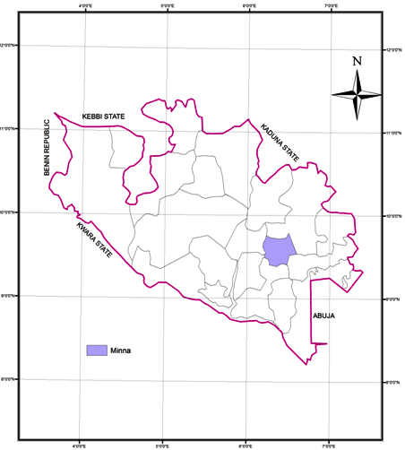 | Figure 1(a). Administrative Map of Niger State showing Minna. (Source: Niger State Ministry of Lands) |
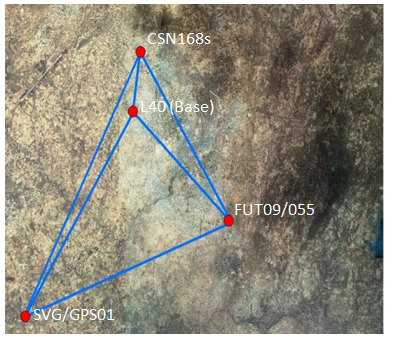 | Figure 1(b). Observed stations for the study |
1.4. Location and Scope of Study
1.4.1. Location of Project
The project site was located in Minna, the capital of Niger state. The city is with an estimated population of over 347,788 and land area of about 6.784 square kilometres. Minna lies between latitudes 9030’00’’ and 11030’00’’ North of the Equator and longitudes 6030’00’’ and 7030’00’’ East of the Meridian, on a geological base of copper, iron, lead, silica, clay, sand, etc (Niger State Diary, 2010). The stations were carefully selected to cover the major axes of Minna, as they are located at House of Assembly Quarters (09/FUT/055), Tudun Fulani (CSN168s), Gidan-Kwano campus of Federal University of Technology Minna (SVG/GPS/01/2008), and at Minna-L40 datum. Figure 1 shows the map of the study area, with the stations in red.
1.4.2. Scope of Project
The scope of this project covers data collection using DGPS (Differential GPS) technique and the estimation of dry tropospheric delay in the data using appropriate models computed with a Java Program. This project does not cater for the wet tropospheric component and other error sources in GPS observation.
2. Conceptual Framework
2.1. Differential Global Positioning System (DGPS)
The DGPS is an enhancement to Global Positioning System that uses a network of fixed, ground-based reference stations to broadcast the difference between the positions indicated by the satellite systems and the known fixed positions. These stations broadcast the difference between the measured satellite pseudoranges and actual (internally computed) pseudoranges, and receiver stations may correct their pseudoranges by the same amount. The correction signal is typically broadcast over UHF radio modem[11]. DGPS data collection can be by static, stop-and-go, and kinematics modes. The three modes run independently. In the Static data collection mode, the GPS receiver systems simultaneously collect raw data from all available satellites while remaining stationary on their respective points. In the Stop-and-Go data collection mode, the GPS receiver systems simultaneously collect raw data from all available satellites while stationary on their respective points and while moving between points. In the Kinematics data collection mode, the GPS receiver systems simultaneously collect raw data from all available satellites while a receiver is moving[10] about 100km above it. The lower part of this shell, ranging from the surface of the Earth to approximately 50km above it, contains about 99.9% of all atmospheric mass. It consists of the troposphere (0-10km), in which temperature decreases with height, the tropopause (10km), at which temperature remains constant, and the stratosphere (10-50km), in which temperature increases with height. The delay experienced by a signal travelling through the neutral part of atmosphere is generally referred to as tropospheric delay, since the troposphere accounts for 90% of the total delay. Therefore, when speaking of the troposphere, often the lower 50km of the Earth's atmosphere is really referred to[8].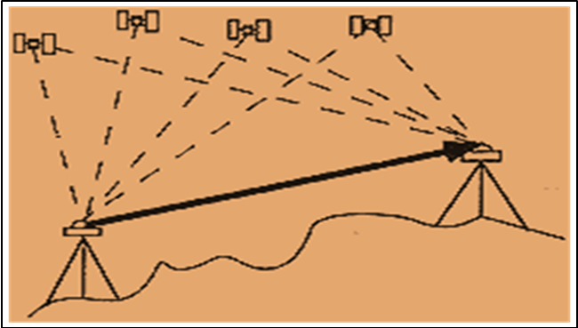 | Figure 2. Principle of DGPS Observation |
2.2. Troposphere
The neutral (non-ionized) atmosphere is an approximately spherical shell extending outward from the Earth's surface to The tropospheric effect is a further factor elongating the runtime of electromagnetic waves by refraction. The reasons for the refraction are different concentrations of water vapour in the troposphere, caused by different weather conditions. The error cannot be eliminated by calculation. It can only be approximated by a general calculation model[16]. The tropospheric delay is separated into two components: dry and wet. The dry component is determined with high accuracy by many tropospheric delay models derived from surface measurements. The wet component, however, is difficult to predict because water vapour is highly variable in space and time such that the wet delay cannot be modelled using surface measurements very accurately[1]. The wet component of the delay constitutes less than 10% of the total effect; tropospheric effect on GPS signals is approximately ± 0.5m[8]. Figure 3 shows the various layers of the atmosphere and the response of air temperature to increasing altitude.
2.2.1. Hydrostatic Models
Early efforts to determine corrections for radio propagation delay by the atmosphere were prompted by the need for improvements in satellite tracking from ground stations.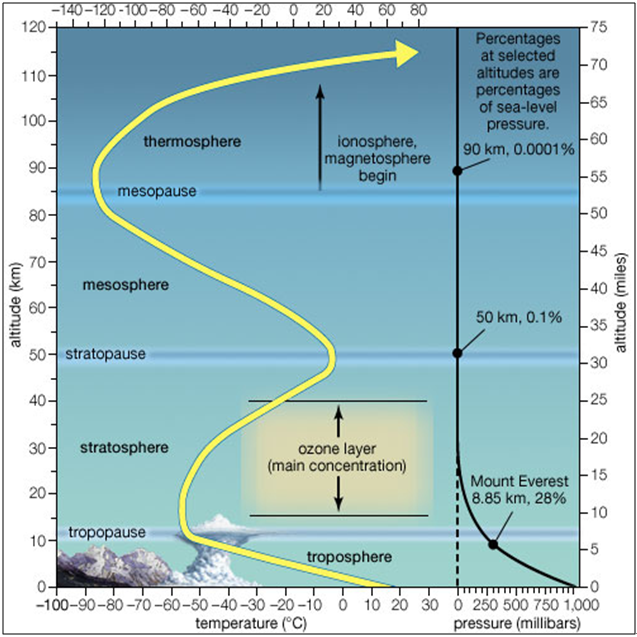 | Figure 3. The Layers of Earth's Atmosphere. Source:[5] |
[13],[12], and[2] made significant contributions to the study of range corrections. Saastamoinen’s Zenith hydrostatic delay and the form of Marini’s approximation for the mapping function for a horizontally stratified refractive medium are incorporated in many current models used for accurate space-based geodetic measurements.[13] Showed that the delay in the zenith direction due to the atmospheric constituents in hydrostatic equilibrium is accurately determined by measuring the surface pressure and making corrections for the latitude and height above sea level of the site from which the observation was made. His formula (or slightly more precise form given by[3] provides the zenith hydrostatic path with accuracy better than 1mm under conditions of hydrostatic equilibrium.[15] investigated the impact of different standard tropospheric models (namely, Saastamoinen model, Hopfield model and Simplified Hopfield model) on GPS baseline accuracy, in order to determine the best-fit standard tropospheric model in Thailand with the GPS data collected in Thailand.The results indicated that there are no statistically significant differences in the performance of the three tropospheric models. However, the use of the Saastamoinen model tends to produce more reliable results than the use of the other two models[15].(i). Saastamoinen ModelIf hydrostatic equilibrium is assumed, the hydrostatic delay model may be expressed simply as a function of measured surface pressure.[14] employed this approach and used the following representation of gravity gm in the zenith hydrostatic model. | (1) |
Where,  is the latitude of the station and
  is the station height above sea level, in metres. Saastamoinen used K1 refractivity constant given by[3] to determine the following expression for the zenith hydrostatic delay:
 | (2) |
where,  is the surface pressure and K1 = 0.0022768.The most stable tropospheric model for the equatorial region is the Saastamoinen Model[15]. Consequently, Saastamoinen Model has been adopted as the Standard dry Tropospheric delay Model for this research.(ii). Davis et al. ModelThe[4] model slightly differs from the Saastamoinen model. Davis el al. used the K1 refractivity constant given by[20] and the zenith hydrostatic model is given by the following expression:
 | (3) |
where,  is the surface pressure and K1 = 0.0022768.(iii). Hopfield Model[7] assumed that the theoretical dry refractivity profile could be expressed using a quartic model:
 | (4) |
where, 
 is the dry refractivity on the surface obtained using the K2 refractivity constant determined by[17] as
  and H is the height above sea level, in metres hence, the final expression for the zenith dry delay can be represented by the following expression:
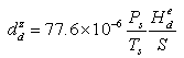 | (4.1) |
where,  is the surface pressure, and
  is the surface temperature and K2 is 2.29286.(iv). Altshuler and Kalaghan (A&K) ModelUsing the K2 refractivity constant determined by[17], the tropospheric delay correction (Δ) in metres is given by[18]:
 | (5) |
where,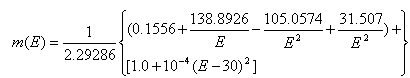 | (5.1) |
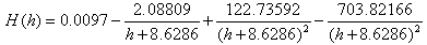 | (5.2) |
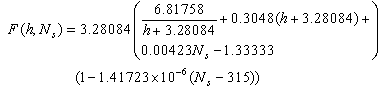 | (5.3) |
 elevation angle in degrees
 height above sea level in metres
 global surface refractivity
 surface pressure in milibars
 surface temperature in degree KelvinK2 = 2.29286m(v). Saastamoinen Model (Using Ground Meteorological Data)Using the K1 refractivity constant determined by[4], the tropospheric delay using this model is given by[18]:
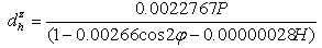 | (6) |
where,  is the atmospheric pressure,
  is the latitude of the station and H is the height of the station above sea level, K1 is 0.002277 in metres.
3. Methodology
During planning, the stations were carefully selected to cover the major axes of Minna using the city map of Minna. The stations are 09/FUT/055 at House of Assembly Quarters, CSN168S at Tudun Fulani, SVG/GPS/01/2008 at Gidan-Kwano campus of Federal University of Technology Minna, and L40 Nigerian datum (base station) see fig. 1 above. The coordinates of the selected stations were collected from the Department of Surveying & Geoinformatics, Federal University of Technology Minna. The details are as shown in the table below:| Table 1. Existing Coordinates of Stations Used |
| | STATIONS | NORTHINGS (m) | EASTINGS (m) | HEIGHT (m) | | L40 | 1066041.870 | 227423.232 | 279.603 | | CSN168S | 1069224.788 | 227914.615 | 306.646 | | FUT 09/055 | 1060188.295 | 233413.820 | 268.390 | | SVG/GPS/01 | 1055093.618 | 220563.650 | 234.138 |
|
|
3.1. Data Acquisition Procedure
Thales ProMark3 Single Frequency DGPS Receivers and the Accessories were used. The static DGPS procedure was used for the field operation. The instrument was set at Minna-L40 datum, which was adopted as the base station. All necessary adjustments were carried out before the necessary parameters were entered into the receiver to start observations. The other three stations were similarly set up and were simultaneously log on to capture data concurrently for an hour, four sets of hourly observation was made during each session.This simultaneous observations were made at all stations between 8:30a.m and 12 noon for morning observation, 2:00p.m and 5:00p.m for afternoon observation, 6:00p.m and 9:00p.m for evening observation. 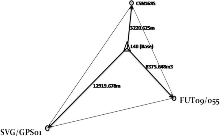 | Figure 4. Network design |
3.2. Data Processing
Since the ProMark3 System operates in conjunction with GNSS Solutions, the acquired field data were processed using GNSS solutions Software. Also, a Java 1.6.0_15 based Program was developed using the selected dry tropospheric delay models. The Java program runs with an installed My SQL Administrator (version 1.1.9) and Net Beans IDE (6.5). The equations defining the models were coded into the program with SQL for fast, efficient and error-free processing to obtain the tropospheric delay.
4. Results and Analysis
4.1. Results
Below are the mean coordinates obtained from the field observations.| Table 2(a). Coordinates of Occupied Stations during Morning Observations |
| | Point ID | Easting(m) | Northing(m) | Height(m) | | L40 | 227423.232 | 1066041.870 | 279.603 | | FUTO9/055 | 233413.977 | 1060188.317 | 268.620 | | GPS01 | 220563.610 | 1055093.227 | 238.305 | | CSN168s | 227913.915 | 1069224.587 | 307.922 |
|
|
| Table 2(b). Coordinates of Occupied Stations during Afternoon Observations |
| | Point ID | Easting(m) | Northing(m) | Height(m) | | L40 | 227423.232 | 1066041.870 | 279.603 | | FUT09/055 | 233413.995 | 1060188.311 | 268.673 | | GPS 01 | 220563.586 | 1055093.221 | 238.245 | | CSN168s | 227913.925 | 1069224.574 | 308.025 |
|
|
| Table 2(c). Coordinates of Occupied Stations during Evening Observations |
| | Point ID | Easting(m) | Northing(m) | Height(m) | | L40 | 227423.232 | 1066041.870 | 279.603 | | FUT09/055 | 233414.011 | 1060188.315 | 268.694 | | GPSS01 | 220563.760 | 1055093.165 | 238.262 | | CSN168s | 227913.901 | 1069224.557 | 308.020 |
|
|
Tables 2(a, b, c) above show the processed three– dimensional (X, Y, Z) coordinates of the occupied stations during morning, afternoon and evening observations using GNSS Solutions.Tropospheric delay affects mainly the height components [19]. Hence, table 3 below shows the mean observed heights at the various occupied stations during observations.| Table 3. Summary of Observed Heights |
| | Statn | Epoch | L 40 | FUT 09/055 | SVG/GPS01 | CSN168S | |
| Observed Heights(m) | Morning | 279.603 | 268.621 | 238.305 | 307.920 | | Afternoon | 279.603 | 268.673 | 238.245 | 308.025 | | Evening | 279.603 | 268.694 | 238.262 | 308.020 | | | Mean of Means | 279.603 | 268.663 | 238.271 | 307.988 |
|
|
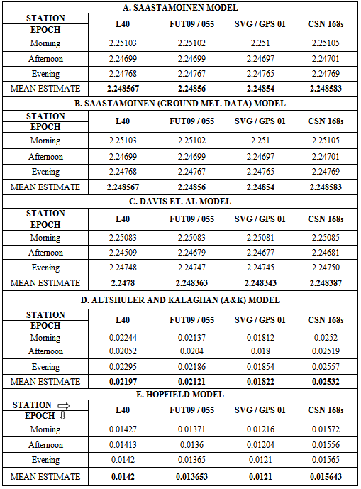
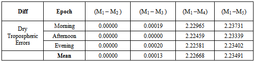
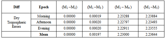
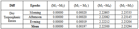
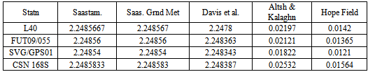
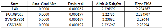
Tables 4 (a to E) below show the dry tropospheric errors estimated by the different tropospheric models during morning, afternoon and evening observations.Tables 5, 6, 7, 8 below show the deviations of the tropospheric delay estimated by the other dry tropospheric models from the adopted standard model (Saastamoinen model) at each station.♦ KEY:M1: SAASTAMOINEN Model, M2: SAASTAMOINEN Model (GROUND MET. DATA), M3: DAVIS, M4: Altshuler and Kalaghan (A&K) Model and M5: HOPFIELD Model ♦ NOTE: Standard Model adopted is Saastamoinen Dry Tropospheric Model[15].Chart 1 below shows graphically, the deviations of tropospheric error estimated by other tropospheric delay models at L – 40 datum in the above table.The Chart 2 below shows graphically, the deviations of tropospheric error estimated by other tropospheric delay models at FUT09/055 station in the above table.The Chart 3 below shows graphically, the deviations of tropospheric error estimated by other tropospheric delay models at SVG/GPS01 station in the above table.The Chart 4 below shows graphically, the deviations of tropospheric error estimated by other tropospheric delay models at CSN168s station in the above table.Table 4. Dry Tropospheric Error Estimates by Each Model per station
 |
| |
|
Table 5. Deviation of Other Models from the Standard Dry Tropospheric Model at L-40
 |
| |
|
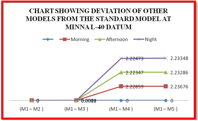 | Chart 1. Deviation of Other Models from the Standard Model at L-40 |
Table 6. Deviation of Other Models from the Standard Dry Troposheric Model at FUT09/055
 |
| |
|
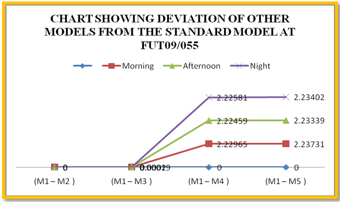 | Chart 2. Deviation of Other Models from the Standard Model at FUT09/055 |
Table 7. Deviation of Other Models from the Standard Dry Troposheric Model at SVG/GPS01
 |
| |
|
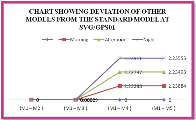 | Chart 3. Deviation of Other Models from the Standard Model at SVG/GPS01 |
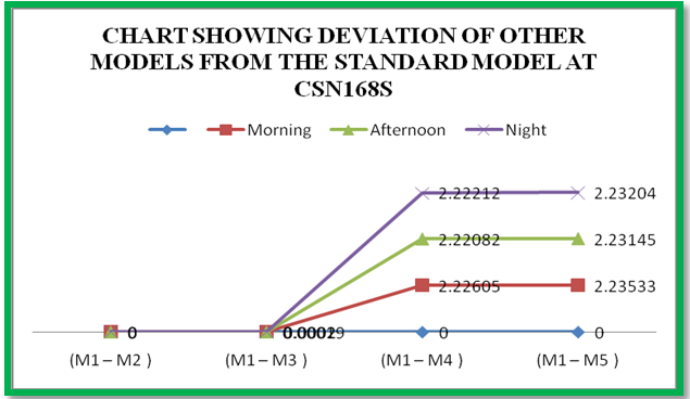 | Chart 4. Deviation of Other Models from the Standard Model at CSN168S |
Table 8. Deviation of Other Models from the Standard Dry Troposheric Model at CSN168S
 |
| |
|
Table 9. Mean Estimate of tropospheric error per station per model
 |
| |
|
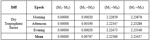
Table 10. Mean deviation per station per model
 |
| |
|
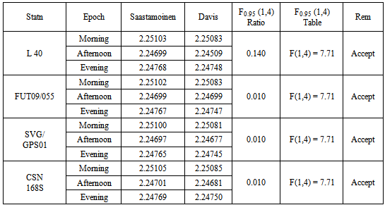
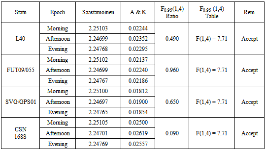
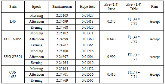
In a further investigation, the hypothesis test was carried out to find out if the differences in the performance of the five (5) standard tropospheric Models at each station are statistically significant at 5% significance level using StatextV1.0 software.The hypothesis is as follows:H0: µ1 = µ2 = µ3 (Null hypothesis)H1: at least two are not equal (Alternative hypothesis)Reject F, if F0.95 > F-Table, otherwise accept null hypothesis.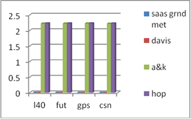 | Chart 5. Mean deviation |
Table 11. Test of Significant Difference between Saastamoinen Model & Davis et al. Model
 |
| |
|
Table 12. Test of Significant Difference between Saastamoinen Model & Altshuler & Kalaghan (A & K) Model
 |
| |
|
Table 13. Test of Significant Difference between Saastamoinen Model & Hopfield Model
 |
| |
|
4.2. Analyses of Results
In the following analyses, the discrepancies in the dry tropospheric errors obtained by the five tropospheric models at various observation epochs are discussed. It can be seen from Tables 2, 3 and 4 above showed that Hopfield Model has the lowest dry tropospheric delay estimates numerically while the highest dry tropospheric estimates are from Saastamoinen and Saastamoinen (Using Ground Meteorological Data) Models. The performance of Saastamoinen, Saastamoinen (Using Ground Meteorological Data) and Davis et al. standard tropospheric Models are very close as their dry tropospheric errors differ only by a few centimetres during morning, afternoon and evening observations, while Altshuler and Kalaghan (A&K) Model and Hopfield Model have centimetre variations among each other but differ from the other three by about two metres (2m). The reason for this is that Saastamoinen, Saastamoinen et al. standard tropospheric Models used the same empirically determined refractivity constant (k1), while Altshuler and Kalaghan (A&K) Model and Hopfield Model used the same empirically determined refractivity constant (k2). Also, it can be seen that there are no variations in the dry tropospheric errors estimated by Saastamoinen Model and Saastamoinen Model (Using Ground Meteorological Data) during morning, afternoon and evening observations. Tables 5, 6, 7, 8 and Charts 1, 2, 3, 4 depicted the absolute deviations of the dry tropospheric Models from Saastamoinen Model which was adopted as the standard Model [15] at each station. This gave the idea of the temporal variability of the estimated tropospheric error by the models. Since Saastamoinen Model (Using Ground Meteorological Data) is highly correlated with the adopted standard model because of the model similarity, the remaining three models were evaluated. It was observed from the tables and the charts that Davis et al. Model gave more consistent results, followed by Hopefield model then Altshuler and Kalaghan (A&K) Model. Furthermore, from the mean estimate in table 9 and the mean deviation in table 10, the standard error of 0.285mm, 1.446mm and 2.899mm were respectively obtained for Davis et al. Model, Hopefield model and Altshuler and Kalaghan (A&K) Model.Finally, from tables 11, 12, 13, the F-test showed that the differences in the performance of the standard tropospheric Models at each station are not statistically significant at 5% significance level.
5. Conclusions and Recommendations
5.1. Conclusions
Total zenith delays and gradient parameters can be estimated with the present GPS data processing. The zenith hydrostatic delay can be accurately inferred from precise measurements of atmospheric parameters. The magnitude of the estimated hydrostatic delay at a particular station depends on the hydrostatic delay model used and the time of observation. Based on the F-test performed, all the Models, i.e. Saastamoinen Model, Saastamoinen Model (Ground Meteorological Data), Davis et al. Model, Altshuler and Kalaghan (A&K) Model and Hopfield Model, generally produced results that are not statistically different. But comparatively, the Davis et al. Model with a standard error of about 0.3mm gave a better performance close to the adopted standard model, i.e. Saastamoinen Model. However, a standard deviation of about 1.4mm and 2.9mm for Hopefield and Altshuler and Kalaghan (A&K) Models respectively corroborate with the statistical test above. It could therefore, be concluded that either of the five models evaluated in this study can perform well in the study area, nevertheless, the choice of Saastamoinen Model, Saastamoinen Model (Ground Meteorological Data) and Davis et al. Model will be more preferable.
5.2. Recommendations
The following recommendations are made based on the research findings:1. The best time for GPS observations with least tropospheric effect are between 2p.m and 6p.m. Also, observations at evening between 6p.m and 9p.m can be made as the tropospheric effect is not high during those times. However, observations at periods when the sun is said to be at its peak (11a.m to 1p.m) should be avoided.2. Further researches like seasonal variations of tropospheric delay, the use of Continuously Observing Reference Stations (CORS) to investigate tropospheric impact, etc, should be encouraged for broader and better understanding of tropospheric effects.
References
| [1] | Bevis, M., S. Businger, S. Chiswell, T.A. Herring, R.A. Anthes, C. Rocken and R. Ware (1994): GPS Meteorology: Mapping Zenith Wet Delays Onto Precipitable Water, Journal of Applied Meteorology, Vol. 33, pp. 379-386. |
| [2] | Chao, C.C. (1972): A Model for Tropospheric Calibration from Daily Surface and Radiosonde, Balloon Measurement, Jet Propulsion Laboratory, Pasadena, California, Technical Memorandum 391-350, pp. 16. |
| [3] | Davis, J.L., T.A. Herring, I.I. Shapiro, A.E.E. Rogers and G. Elgered (1985): Geodesy by Radio Interferometry: Effects of Atmospheric Modelling on Estimates of Baseline Length, Radio Science, Vol., 20, No. 6, pp. 1593-1607. |
| [4] | Essen, L. and K.D. Froome (1951): The Refractive Indices and Dielectric Constants of Air and Its Principal Constituents at 24, 000 Mc/s. Proceedings of the Royal Society B, Vol. 64, pp. 862-875. |
| [5] | Encyclopaedia Britannica (2009): Student and Home Edition. |
| [6] | "Global Positioning System"(2010). www.gps.gov |
| [7] | Hopfield, H.S. (1969): Two Quartic Troposheric Refractivity Profile for Correcting Satellite Data, Journal of Geophysical Research, Vol.74, No. 18, pp. 4487-4499. |
| [8] | Hopfield, H.S. (1971): Tropospheric Effect on Electromagnetically Measured Range: Prediction from Surface Weather Data, Radio Science, Vol. 6, No. 3, pp. 357-367. |
| [9] | Janes, H.W., R.B. Langley and S.B. Newby (1991): Analysis of Tropospheric Delay Prediction Models: Comparisons with Ray Tracing and Implications for GPS Relative Positioning, Bulletin Geodesique, Vol. 65, No. 3, pp. 151-161. |
| [10] | Kaplan, E. D. and Hegarty, C.J. (2006): Understanding GPS; Principles and Applications, 2nd edition. Artech House, Inc. |
| [11] | Lachapelle, G. (2001): Advanced GPS Theory and Applications, ENGO 625 Course Lecture Notes, University of Calgary, Calgary, Canada. |
| [12] | Marini, J.W. (1972): Correction of Satellite Tracking Data for an Arbitrary Tropospheric Profile, Radio Science, Vol. 7, No. 2, pp. 223-231. |
| [13] | Saastamoinen, J. (1972): Atmospheric Correction for Troposphere and Stratosphere in Radio Ranging Of Satellites, Geophysical Monograph, 15, American Geophysical Union, Washington, D.C., pp. 247-252. |
| [14] | Saastamoinen, J. (1973): Contribution of the Theory of Atmospheric Refraction, Bulletin of Geodesique, No. 105, pp. 279-298, No. 106, pp. 383-397, No. 107, pp. 13-34. |
| [15] | Satirapod, C., Chalermwattanachai, P. (2004): Impact of Different Tropospheric Models on GPS Baseline Accuracy: Case study in Thailand. A paper presented at the 2004 International Symposium on GNSS/GPS. |
| [16] | Skone, S., M. El-Gizawy and S. M. Shrestha (2001): “Limitation In GPS Positioning Accuracies And Receiver Tracking Performance During Solar Maximum”, Proceeding of KIS, Banff, Canada. |
| [17] | Smith, E.K. and S. Weintraub (1953): The Constants in the Equation for Atmospheric Refractive Index at Radio Frequencies. Proceedings of I.R.E., Vol. 4, pp. 1035-1037. |
| [18] | Spilker, J. J. (1996): Global Positioning System: Theory and Applications; “Tropospheric Effects on GPS”, Chapter 13, Volume I, The American Institute of Aeronautics and Astronautics, Inc., Washington, D.C. |
| [19] | Sudhir M. S. (2003): Investigations into the Estimation of Tropospheric Delay and Wet Refractivity Using GPS Measurements, Unpublished Master’s Thesis, Geomatics Engineering Department, University of Calgary, Alberta, Canada. |
| [20] | Thayer, G.D. (1974): An Improved Equation for the Radio Refractive Index of Air, Radio Science, Vol. 9, No. 10, pp. 803-807. |
 Abstract
 Reference
 Full-Text PDF
 Full-text HTML