Carl Y. H. Jiang
Centre for Intelligent Systems Research, Deakin University, Victoria, 3216, Australia
Correspondence to: Carl Y. H. Jiang, Centre for Intelligent Systems Research, Deakin University, Victoria, 3216, Australia.
| Email: |  |
Copyright © 2012 Scientific & Academic Publishing. All Rights Reserved.
Abstract
Bushfire has been classified into several burning zones for easily modeling according to remote sensing imagery. Estimating mass and heat transport released from an individual large scale bushfire has been implemented in detail by means of integrating knowledge of transport phenomena with hybrid technique of combining features of digital elevation model and remote sensing imagery. The multi-component smoke has been treated as single-component substance. Mass diffusion takes place in a smoke –air binary system. The effective semi-infinite model has been effectively selected. The basic theories in mass diffusion and heat conduction has been reviewed and applied into calculating distribution of pollutant concentration and temperature profile of bushfire, and analysing emission rate of mass and energy using one chosen geographical location respectively.
Keywords:
Bushfire Modeling, Digital Elevation Model, Satellite Imagery, Mass and Heat Transport
Cite this paper: Carl Y. H. Jiang, Estimate Mass and Heat Emitted from Bushfire Based on Digital Elevation Model and Remote Sensing Imagery, American Journal of Geographic Information System, Vol. 2 No. 4, 2013, pp. 108-120. doi: 10.5923/j.ajgis.20130204.04.
1. Introduction
The experimental modelling bushfire has been investigated by many researchers[1-4]. However, so far several knowledge of burning process for bushfire has not been fully understood. Over last a few years, researchers started to draw their attention to studying bushfire by means of remote sensing technology. The energy emitted from bushfire transports through air in the form of radiation, which can be measured by the instrument of Moderate Resolution Imaging Spectro-radiometer (MODIS) installed in satellites. In the bushfire research, Wooster and co-operators[5] have provided a series of valuable data from Sydney bushfire on 5 January 2002 in estimating bushfire energy. Other concerned topic is that how much degree of temperature of bushfire can maximally reach to. Such research has been reported by Dennison[6], they have found that the temperature of bushfire can range from 500 to1500K according to Visible Infrared Imaging Spectrometer (AVIRIS) data. However, the application of the experimental modelling and two dimensional satellite imagery studies is confined. In order to overcome existing deficiency in the technique of investigating bushfire, a novel research method is to be proposed in this paper with detailed demonstration. Features of ResearchFollowing up the previous in modelling bushfire[7, 8], in this research paper, the novel technique of integrating features of digital elevation model (DEM) and remote sensing imagery is used to combine semi-infinite model mathematically generated from transport phenomena to explore the characteristics of bushfire in mass and heat transport.Objectives and Scope of Research The goal of this research is to be performed in the following fields.1. What the mass and heat transport physically mean in describing transport phenomena of substance (thus smoke).2. How the mass and heat transport are expressed mathematically.3. What coefficients are used in describing the properties of substance, what roles they play in determining the physical properties generated in mass and heat transport.4. How calculating distribution of pollutant (smoke) concentration and temperature profile of bushfire in different case is carried out.5. How the emission rate of mass and energy is estimated respectively.6. How the burning surface area is assessed by using selected geographical location. Bushfire is a very complicated process, it is difficult to decide some coefficients used in modelling and accurately acquire them from bushfire place. In fact, deciding mass and thermal coefficients (such as mass diffusivity, thermal diffusivity) with varying multi-components at different temperatures and pressures is an extremely difficult work. For the sake of simplicity and effectiveness, in this research, those coefficients are chosen from some engineering hand books[9, 10] in virtue of one pure substance (e.g. CO2) at a constant pressure (1 atm). However, those data themselves are collected from other different sources. They are usually classified into two types: theoretical calculation and experiment. Therefore, in practice, those data are treated as reference ones and must be adjusted and modified according to the specific cases happening in bushfire.Based on above, the results gained from modelling are already able to sufficiently explain some phenomena occurred in bushfire spread in landscape. The physicochemical properties for multi-component smoke are therefore not taken into account; instead, in the process of treatment, the smoke is in general regarded as a single-component substance in this research.
2. Methodology
Assessing local distribution of temperature and concentration is most important for the fire-fighter, residents and government. In studying bushfires, the temperature and concentration of smoke can be assessed using semi-infinite slab model with a constant or dynamic heat flux. Although a burning zone consists of many burning spots, each burning spot can be arbitrarily treated as one burning zone having any size area (see Figure 17 ) to study. Such a treatment does not affect the quality of modelling because the calculation relies on the geometric information such as surface area. Its detailed method has been introduced by author[8].For the sake of simplicity, each of burning zones can be treated as a place to supply either a constant heat source within a certain time (See Figure 1) or a time-variation heat resource. The similar treatment is also applied to mass transport, which is to be discussed after heat conduction.In terms of the characteristics of bushfire, the semi-infinite model to be briefly introduced in the following sections is much closer to the real case of bushfire in landscape. Because there are massive concepts of engineering mathematics involved in the following introduction, the valuable references[10, 11] should be considered for seeking for more details. All calculations are implemented by MATLAB®.Transient Heat Conduction
2.1. Fourierian Second Law
Based on the Fourier’s second law, the heat conduction generated by bushfire in one direction can be expressed as  | (1) |
In which variable T , t and z denote temperature, time and displacement or distance in z-direction at a three dimensional coordinates(see Figure 1) respectively.In which α is the thermal diffusivity of one substance. | (2) |
In which k is the thermal conductivity of one substance to indicate its ability to conduct heat, ρ is its density and Cp is its heat capacity at constant pressure denoted by subscript p in the context; the term ρCp tells the ability of the substance to absorb heat. The lager the thermal diffusivity α is, the faster the heat transport happens.Also the smoke in this paper is assumed as an isotropic media in the context, so that heat is conducted with the thermal conductivity in all directions.
2.2. Heat Flux
The heat flux expresses how fast the energy released from heat source, its unit is [energy] per [area] [time]. It is often defined as follows in one-dimensional form.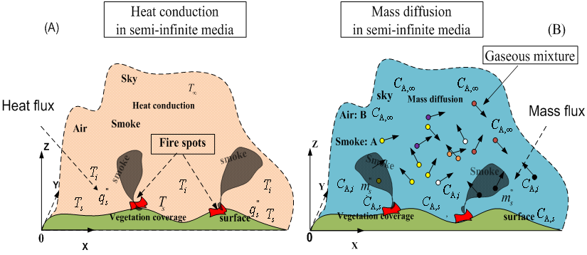 | Figure 1. schematic presentation of concentration and temperature distribution over terrain |
 | (3) |
In fact, the equation (3) is one-dimensional version of the Fourier first law. When z=0, the heat flux q”(0,t) is simply rewritten as qs”, the subscript s denotes surface, thus indicates that the heat flux takes place at the surface. It is similar to other cases in the context.
2.3. Temperature Distribution
If the temperature T jumps from the initial temperature Ti to the surface temperature Ts, when Ts> Ti thus the surface is heated ,then the distribution of temperature T between ground and sky (see Figure 1) can be expressed as  | (4) |
In which the subscript i denotes the initial condition in the context and the erfc is the complementary error function in mathematics with the mathematical properties of erfc(0)=1, erfc(∞)=0 and  In which the erf is the error function having following mathematical property
  | (5) |
erf(0)=0, erf(∞)=1.The equation(5) is very useful in the procedure of the mathematical derivation especially in Laplace transform.
2.4. Temperature Distribution with Constant Heat Flux Source
However assigning the following initial, boundary, and auxiliary condition (thus I.C., B.C., A.C. shown in the condition of (6) ) into equation(1) , | (6) |
It produces a temperature distribution of the semi-infinite model shown in the equation(7) with constant heat flux qs”. | (7) |
Because  and
and , the temperature distribution at the ground surface is simplified as follows.
 | (8) |
In the mathematical derivation of equation(7), the heat flux qs” is treated as a constant. However, in the process of modelling, it is technically able to be treated as a function of time to the meet specific requirement of one case.
2.5. Total Energy Emission Rate in Burning Zone
The total energy emitted by bushfire is a process of accumulating the amount of energy released by the burning vegetation with respect to time. To acquire the total energy emission rate in a given burning zone, combining the equation(3), (4)and (5) yields  | (9) |
At the surface, thus z=0, the heat flux  is shown as
  | (10) |
Therefore, the total energy emission  from the ground is calculated from time 0 to t by equation(10). It yields
 | (11) |
In which S is the area of one substance being produced, in this case, it can be interpreted as the surface area of burning zone. Transient Mass Diffusion
2.6. Fickian Second Law
Due to the similarity between mass and heat transport in the differential equations, initial and boundary conditions, being analogous to equation(1), the one-dimensional version of Fick’s second law can be expressed as | (12) |
In which CA is the concentration of substance A, the DAB denoted by the subscript A and B respectively in the context is the binary mass diffusivity of the mixture of substance A and B. This parameter indicates how fast the diffusion of substance A and B takes place in the A-B binary system and has an analogy with thermal diffusivity mentioned previously. The unit is[length]2 per[time]. Because the mass diffusion between substance A and B in the binary system happens independently, DAB is equal to DBA.
2.7. Mass Flux
Being similar to the equation(3), the mass flux in terms of the one-dimensional Fick’s first law can be expressed as | (13) |
In which  is mass fraction of the mass of substance A plus the mass of substance B in a given microscopic volume element.
  is the density of the A and B system. In the case of modelling bushfire, to simplify the complexity of case, the substance A and B can represent smoke mixture and air respectively. Thence, when smoke disperses from ground into air at the initial stage, its behaviour is treated as binary diffusion in a semi-infinite system (landscape-sky system).
2.8. Concentration Distribution with Constant Surface
Similarly, the concentration distribution of substance A can be expressed by equation(14). The boundary condition of it is that the initial concentration CAi jumps to CAs, and CAs> CAi, then the surface concentration is being maintained as the quantity of CAs for a while. | (14) |
2.9. Concentration Distribution with Constant Mass Flux
According to the Fick’s second Law, the concentration distribution with a constant mass flux source is shown by equation(15). | (15) |
 | Figure 2. one burning zone marked by one circle in modeling |
 | Figure 3. one burning zone marked by one circle in DEM is selected from bushfire spread |
In which  is constant mass flux of substance A. The similar mathematical treatment to
  in one subsection is to be performed in handling it as a function of time so as to describe how it distributes in landscape with respect to location and time.
2.10. Total Mass Emission Rate in Burning zone
Analogically, the total amount of emitted gaseous mixture  with time t is therefore expressed as(16).
 | (16) |
Up to this point, above discussed equations are mathematical expressions which consist of a semi-infinite model and are used in modelling mass and heat transfer for the bushfire happening on the ground. They are already introduced briefly. In the following sections, their applications are to be gradually demonstrated by using individual coefficients, initial and boundary conditions from general cases to geographical information based bushfire modelling.
3. Results and Discussion
The results of modelling to be displayed and discussed are classified into two types: mass and energy based on above equations. Before moving into specific modelling, the chosen geographical information is introduced as follows.
3.1. Geographical Location for Modelling
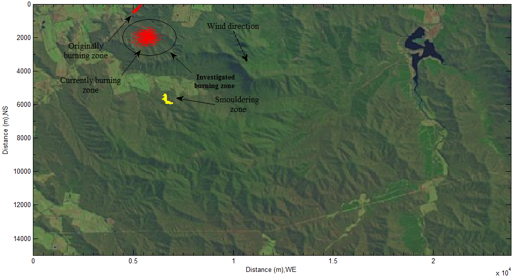
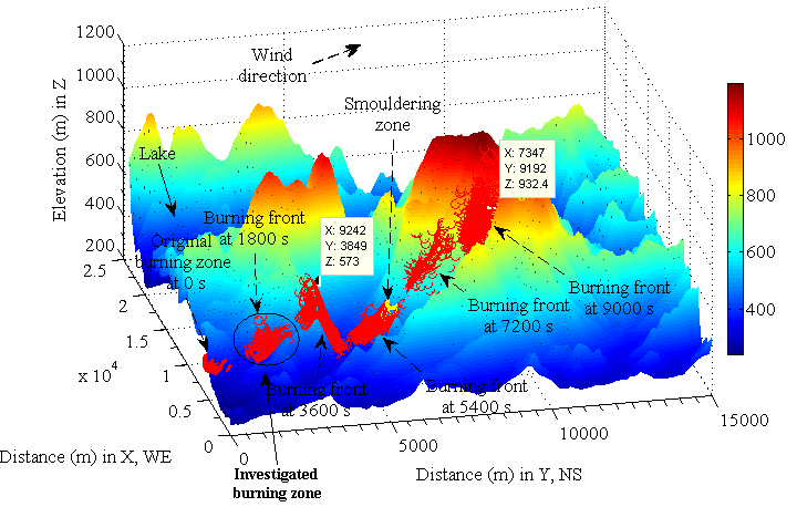
Estimating mass and heat released from bushfire in this modelling is based on the place where bushfire often took place historically in Victoria, Australia. The geographical location (-36°70'10" S, 146°44'30" E; -36°83'60" S, 146°71'00" E) is shown by Figure 2. The distribution of vegetation is stored in the remote sensing imagery captured by the satellite LANDSAT and the feature of terrain is illustrated by the corresponding DEM in Figure 3. In Figure 3, the bushfire spread in landscape downwind was modelled. However, in this research, the concerned topic is to explore mass and heat transport occurring at one burning zone marked by a circle shown in Figure 2 and Figure 3 respectively.General Case Study of Heat ConductionIn the preceding sections, the basic concepts of heat conduction happens in semi-infinite medium in one-dimensional version of Fourier’s second law is already introduced. Before applying yielded equations into estimating the profile of temperature of bushfire and concentration of pollutants and calculating amount of energy and mass is emitted during bushfire spread in one burning zone, it is necessary to consider some general cases so as to further understand some uncertain factors existing in the heat and mass transfer caused by bushfire.
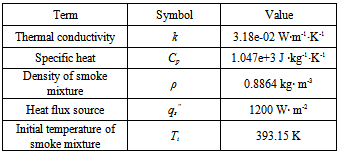
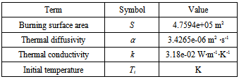
3.2. Common Parameters and Values Used in Calculation of Heat Transport
Some common parameters and their values used in calculation of heat transport are listed in Table 1 besides the ones specified in some case studies in the context. As mentioned previously, some data are collected from source on the basis of carbon dioxide CO2. Due to different conditions of measurement, the values collected by different source are different. However, in this paper, the attention is paid to investigate transport phenomena happening at bushfire by means of some known data obtained in the laboratory scale experiment and to estimate some main physical properties such as temperature of bushfire and concentration of pollutant, which is to be discussed later. Table 1. common parameters and values used in heat transport
 |
| |
|
3.3. Temperature Distribution with Constant Surface Temperature
In the case shown by equation(4), it can be interpreted as that the initial temperature Ti is suddenly raised to one higher surface temperature Ts and Ts is remained for a while. This case could happen in smouldering zone. The ambient temperature jumps to a very high temperature because the vegetation is heated through the heat transport from the heat resource such as smoke plume and solar radiation.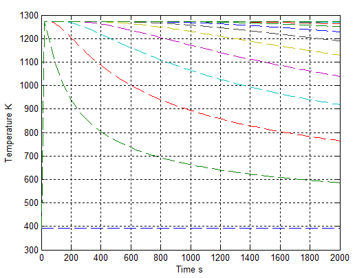 | Figure 4. temperature distribution with condition Ts=1273 K and α = 3.29e-1 m2∙s-1 |
In virtue of the temperature distribution shown in Figure 4, it can be discovered that the temperature after vegetation being burnt is decreased with respect to the time if gaseous mixture has a higher thermal diffusivity α.In other words, the maximum temperature at group surface Ts is being instantly decayed. So-called constant surface temperature is only assigned for mathematical calculation. Its physical meaning in reality is that this temperature is impossible to maintain for a long time for a quick, simultaneous and thermal conduction.
3.4. Temperature Distribution with Increasing Heat Flux and Initial Temperature
The heat flux is defined as the energy pass through one unit area per time. In the bushfire, for any burning area, it must be a place where to generate heat flux when the vegetation is being burnt. In general, the heat flux is increased within initial time interval and then reduced with respect to decreasing amount of fuel (vegetation).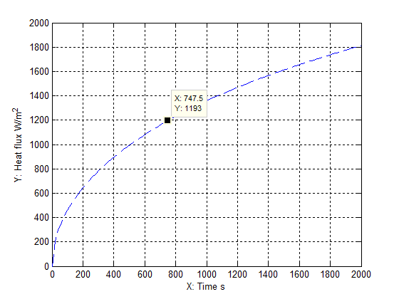 | Figure 5. heat flux is increased with time at an initial stage |
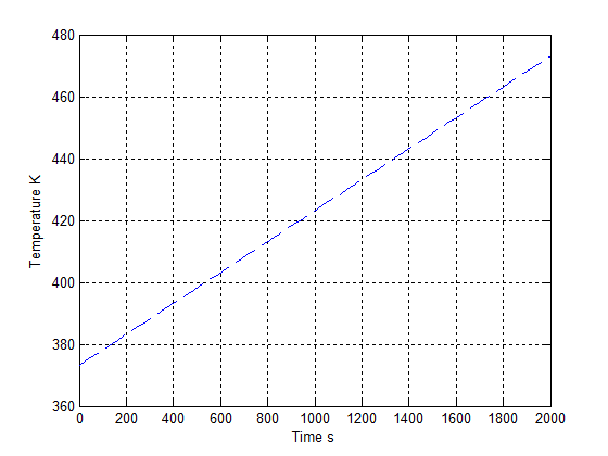 | Figure 6. Initial temperature linearly increases with time |
In Figure 5, the heat flux is assumed to be distributed in each burning zone and increase gradually with time at an initial stage. One heat flux represents one burning zone. The initial temperature of vegetation which is located at different place to be ignited is also assumed to linearly increase with time (see Figure 6). Its temperature range is between 380−470K to represent different ignited temperature for different vegetation ad different location. Applying the data yielded from Figure 5 and Figure 6 into equation(7), the corresponding temperature profile with the increasing time at different location is displayed in Figure 7.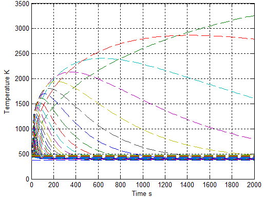 | Figure 7. temperature distributes with increasing heat flux and initial temperature with α = 3.4265e-05 m2∙s-1 |
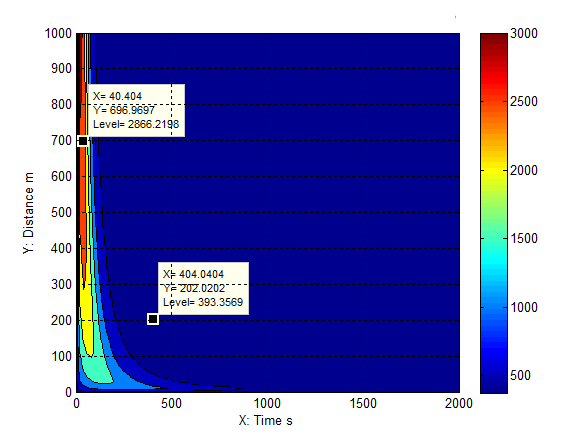 | Figure 8. temperature distributes with increasing heat flux and initial temperature α = 3.4265e-06 m2∙s-1in time and distance profile |
As seen from Figure 7, for a given properties of gaseous mixture with different heat flux, in general, the main feature of each temperature profile is that each temperature increases at the first stage and then reduces when starting from one distinguished iinitial temperature with respect to increasing time. In other words, each temperature profile is displayed by the different heat flux and initial temperature at the different location with respect to individual increasing time. The further illustrating it associated with different location can be obtained from Figure 8. Given one fixed time (e.g. at 40 second), the temperature at one location where the one-dimensional distance is 697 meter can reach up to 2866 K due to the massive energy supplied by one specific heat flux, and then the temperature reduces later. If the location is given (e.g. the point is located at 202 meter), the temperature reduces to be 393 K from one higher temperature (e.g. 1200K) in one time interval. For more details of explanation, it should be carried out by combining it with the three-dimensional result shown in Figure 9. The general approach of heat conduction from each heat flux supplier at ground increases at first and then reduces with respect to increasing time. The degree of temperature decrement is mainly influenced by individual thermal diffusivity α produced by each burning spot.The general conclusion of it is useful in explaining the phenomena during bushfire.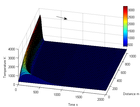 | Figure 9. temperature distribution is displayed in three-dimension |
3.5. Temperature Distribution with Constant Heat Flux at Ground
The temperature distribution with one constant flux at ground calculated by equation (8) is displayed in Figure 10. As expected, the temperature at ground significantly increases under a constant heat flux due to the lower thermal diffusivity α. | Figure 10. temperature distributes with constant heat flux qs”=1200 W∙ m-2 at ground |
Up to this point, it can be found that thermal diffusivity dramatically affects how fast the temperature of one substance (e.g. gaseous mixture) changes within one given binary system. In the following sections, the similar case of concentration is to be discussed. General Case Study of Mass Transport
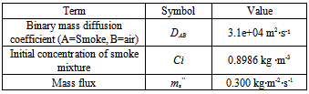
3.6. Common Parameters and Values Used in Calculation of Mass Transport
Although the concentration distribution is analogous to temperature distribution, of most difficulty is to determine the diffusivity of smoke mixture.The mass diffusion in vertical direction is influenced by buoyancy, thermal force, gravitational force and Coriolis force at ground. The resultant force of them drives gaseous mixture rises quickly. In general, in the process of combustion, the concentration at lower level is always larger than the one at higher level at initial stage. In practice, the extensive properties of mass diffusion are mainly influenced by the mass diffusivity. The mass diffusivity is enlarged with increasing temperature. Directly measuring mass diffusivity is very difficult. Instead, for a binary mixture of gases, assuming it has ideal gas behaviour and depends on the pressure (P) and temperature (T), the binary mass diffusion coefficient or diffusivity may be estimated by using the following relation[10].  | (17) |
Provided P = 1 atm, the corresponding results are represented in Figure 11. 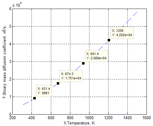 | Figure 11. binary mass diffusion coefficient DAB increases with time |
Table 2. common parameters and values used in mass transport
 |
| |
|
The common used parameters and values in the calculation for mass transfer are listed in Table 2 except for ones specified in some cases in the context.
3.7. Concentration Distribution with Constant Surface Concentration
As explained in the equation(14), the concentration of gaseous mixture jumps from to the lower value Ci to the higher one Cs, and then maintains that value Cs for very a short time.The feature shown in Figure 12 indicates that the distribution of concentration decreases with respect to time. This property states a fact that the concentration of one gaseous mixture reduces with respect to the elapsed time if the diffusion happening between two different gaseous phases is purely caused by the gradient of concentration. 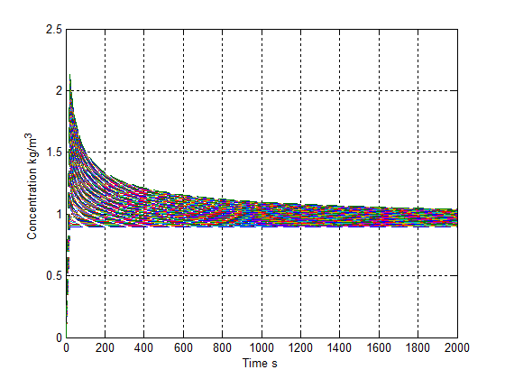 | Figure 12. concentration distribution with Cs =2.864 kg ∙m-3 |
3.8. Concentration Distribution with Increasing Mass Flux and Initial Mass Diffusivity
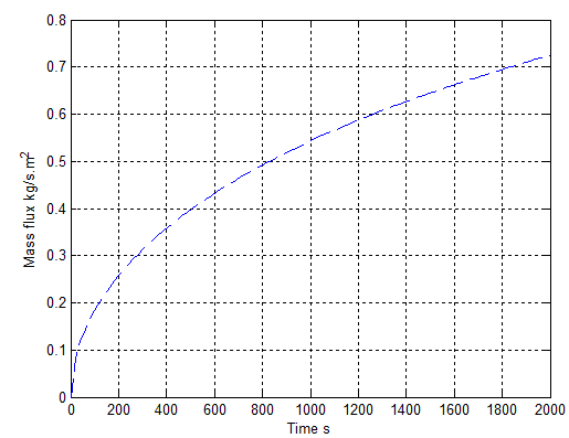 | Figure 13. mass flux increases with time at an initial stage |
In the process of bushfire spread, a burning zone could consist of several burning spots. Like the heat flux mentioned above, a series of mass fluxes located in different positions coexist while the vegetation is burning. In order to demonstrate this approach, an increasing mass flux at each location with time is displayed in Figure 13.However, as illustrated the case of heat flux, each mass flux shown in Figure 13 is considered into the corresponding point of location in the calculation so as to satisfy with the real case happening in bushfire. Similarly, one mass flux represents one burning zone.Applying data from Figure 11 and Figure 13 into equation (15) produces the result of concentration profile at different position with increasing time in Figure 14. The corresponding result with more information is also provided in Figure 15 and Figure 16.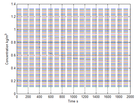 | Figure 14. concentration distributes with increasing mass flux and diffusivity |
It is obviously discovered from Figure 15 and Figure 16 that the concentration at the lower level of each location is the biggest. Its concentration slightly reduces with respect to time. The degree of reducing concentration approaches a constant.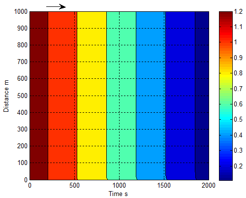 | Figure 15. concentration distributes with increasing mass flux and diffusivity in time and distance profile |
The mass transport is mainly affected by mass diffusivity. According to the relationship between temperature and mass diffusivity shown in the equation(17), the smoke is quickly dispersed accompanying with massive heat emitting as soon as the vegetation is ignited, and then becomes a diluted gaseous mixture in sky in one certain time interval. 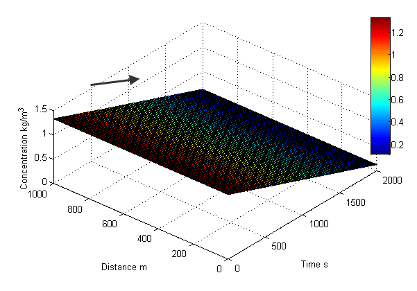 | Figure 16. concentration distribution is displayed in three-dimension |
At this stage, the mathematically modelling general cases of mass and heat transport is already introduced above. In the following sections, the focus of their applications is to be moved to studying the cases on the basis of geographical location.Case Study in Modeling Bushfire
3.9. Temperature Distribution with Constant Heat Flux Combining with Geographical Location
The concept of classifying bushfire burning zone is gained from the scenario shown in remote sensing imagery (see Figure 17). The scale of selected burning zone relies on the concerned spot.As mentioned previously, the specific burning zone selected for modelling is displayed in Figure 2 and Figure 3.The results in Figure 18 represent the temperature distribution occurring in a currently burning zone, which are calculated by the equation(7) using the supplied values of some parameters listed in Table 1.As seen from the case D, the temperature can reach to over 1200 K at the surface of ground if the constant heat flux supplied by bushfire is 1500 W∙m-2. The temperature generated from the calculation is quite consistent with the typical range of 1070 −1470 K reported by Dennison[6]. Very clear, the burning temperature is to be increased if more energy is released. However, even if bushfire in the burning zone is able to supply such constant heat flux, the real temperature may be somewhat lower than the one generated by it according to meteorology, the temperature of 0.98℃ is lapsed per 100 meter ascent[12]. The case of A, B, C and D may represent the process of burning different type vegetation respectively. Because the heat of combustion for different vegetation is different, that results in different heat flux with different profile of temperatures as indicated before.In terms of the distribution of temperature, it may be useful to forecast the bushfire spread and consider how fast the smouldering zone is formed. For instance, assume that the energy dispersion over a given surface is isotropic flux and the boundary in the x or y direction shown by the point a in Figure 18 is treated as the front of bushfire. If the bushfire spreads in landscape downwind, in about 3500 seconds later (in the case A) the bushfire could arrive in the point b according to the temperature displayed at the point b. The direct distance could be 200 meters according to the corresponding point b at Figure 19.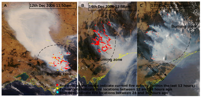 | Figure 17. December 2006 Victorian bushfire satellite images, Australia[13] |
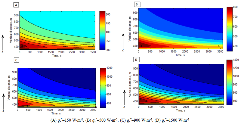 | Figure 18. distribution of temperature vs. burning time and vertical distance |
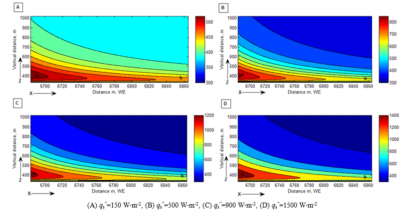 | Figure 19. distribution of temperature vs. horizontal and vertical distance |
Actually, how fast the bushfire spreads depends on how big area of the smouldering zone is formed in advance. Generating the smouldering zone requires continuous energy supply and time. In addition to solar radiation and the radiation coming from smoke plume, the heat transport from the closer bushfire zone is one main energy resource. Under such a situation, the vegetation located in smouldering zone is quickly heated. One part of energy is consumed to evaporate the moisture component from inside vegetation (thus, latent energy of evaporation). That could lead to two possible situations. The one is vegetation in the smouldering zone is self-burning when the temperature of volatile gaseous mixture evaporated from vegetation reaches to its flash point. Based on the temperature indicated in the case D, the vegetation at location b could be self-burning by means of heat conduction in a time interval. Another is that the vegetation is not burnt yet. In case B and C, the vegetation at location b could be satisfied with such a condition within a short time interval. In the former case, the time of bushfire spread is reduced dramatically and bushfire could happen everywhere. In the latter case, it still has time for fighters to extinguish the fire.Another prominent feature which can be found from Figure 18 and Figure 19 is that the temperature profile in sky direction. The elevation of terrain at the point a is approximately 400 meters. Therefore, the temperature profile over bushfire spots varying with the height is useful for pilots to operate their aircrafts safely when they are extinguishing bushfire in sky.
3.10. Concentration Distribution with Constant Mass Flux Combining with Geographical Location
In this section, the concentration distribution is calculated using the equation(15) , the value of parameters is supplied in Figure 20 respectively. In order to illustrate how the temperature affects mass diffusion, the values of temperature are supplied as well.The case A in Figure 20 is the distribution of concentration under the normal temperature, it is not suitable for large scale intensive bushfire at very high temperature. It is only used for comparison. From the case B, C and D, it can be discovered that the concentration is changed slightly when temperature, binary mass diffusivity and mass flux has reached to a certain amount. That is because for a constant heat and mass source existing in the burning zone, the concentration gradient ∂CA /∂z approaches to a constant and ∂CA /∂t≈ constant as well within a limited space and time interval. That tells that mass diffusion approach a steady state. However, in reality (refer to the real case captured by the satellite and shown in Figure 17), the state is kept temporally. The local wind and buoyancy accelerate the diffusion of mass; such temporary equilibrium is immediately broken.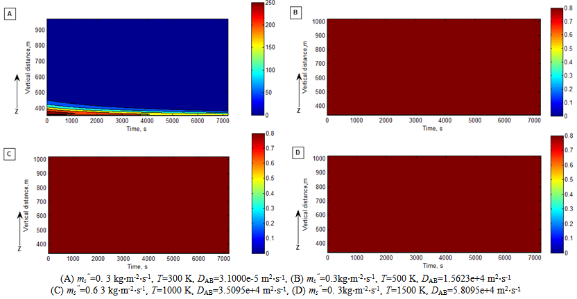 | Figure 20. distribution of concentration vs. burning time and vertical distance |
 | Figure 21. Amount of emitted smoke mixture and amount of energy released from fire vs. burning time |
The results of simulation are useful to estimate how the pollutant is distributed spatially and for pilot and scientist to gain information about the degree of vision and when aircraft is used to extinguish bushfire and consider how the pollutant impact upon bio-environment respectively.
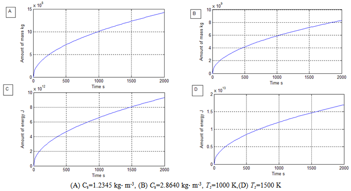
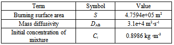
3.11. Emission Rate of Total Mass and Energy
The emission rate of total energy and mass emitted from bushfire (See Figure 2 and Figure 3 ) are calculated by using equation (16) and (11) respectively, and the corresponding data supplied in Table 3 and Table 4. The burning surface area S is the sum of vegetation surface area. The vegetation surface area is classified in the remote sensing imagery (see Figure 2) and indexed before the modelling bushfire is performed in DEM (see Figure 3). In this research, the area of one pixel shown in the remote sensing imagery is equivalent to 25.6m×31.807m in a horizontal plain at ground. Multiplying the secant function against the corresponding slope angle with the unit area, the surface area of vegetation is then obtained[7, 8].The results from (A) to (D) in Figure 21 indicate that massive amount of smoke mixture and energy is instantly emitted by bushfire during its spread in landscape. It dramtically impacts upon envirement and accelerates the bushfire spread. Therefore bushfire belongs to natural disaster for human being. Huge energy and mass of polluant causes a lot of loss including life.Table 3. data used for calculating emitted mass
 |
| |
|
Table 4. data used for calculating emitted energy
 |
| |
|
4. Conclusions
A. Achievements in researchIn this research, several tasks has been achieved and summarized as follows.1. Because bushfire takes place between landscape and infinite sky, the semi-infinite model is then chosen for calculation. So-called semi-infinite model is formed by specifying initial and boundary conditions in the process of finding solution to the second order partial differential equations. The boundary condition in sky is infinite, the corresponding concentration and temperature approaches to zero and temperature in sky respectively. Therefore, this model fits to bushfire well. 2. The physical properties of substance are one of important factors affecting mass and transport. Therefore the values of them used in the research are based on the collected data shown in engineering hand books and suitably adjusted and modified according to the real case.3. To simplify the complex case existing in gaseous mixture (smoke), the mass diffusion between smoke and air is assumed as a binary system, which locates in between ground and infinite sky and takes place within it. 4. The advantage in this research is fully making use of surface area which is accurately supplied by integrating geometric feature of DEM and remote sensing imagery. This is an important standing stone to effectively investigate a large scale bushfire using modelling. On the basis of above, quantitatively calculating mass and heat transport becomes possible and reasonable. 5. In order to simplify the case, the constant heat and mass flux are chosen in the mathematical operation. However, in modelling, they become a function of time individually to indicate different burning zone. The similar treatment is also applied into initial temperature (ignited temperature). 6. The quantity of mass and thermal diffusivity is decided by the physical properties of substances respectively when they represent a specific behaviour in a given system. However, those two parameters play significant role in determining some concerned physical properties such as the distribution of temperature and concentration. The most difficult is directly measuring them from bushfire.7. Massive amount of smoke mixture and energy is emitted by bushfire respectively during bushfire spreads on ground. It seriously pollutes environment and accelerates bushfire spread.The technique provided in this paper is able to not only calculate mass, thermal and other physical properties of bushfire but also reasonably forecast the bushfire spread. The yielded information is useful for the practical guidance in extinguishing a large scale bushfire. B. Future workHaving been able to properly estimate some properties generated by bushfire from ground, at next stage, the further relevant researches will focus on 1. How concentration and heat of smoke is distributed spatially. 2. How the energy carried by the dispersed smoke plume impacts on the vegetation in the smouldering zone.
ACKNOWLEDGEMENTS
Author wants to offer special thanks to Professor Jing. X. Zhao at Shanghai Jiao Tong University for supplying desired data used in this research.
References
| [1] | H. C. Hottel, G. C. Williams, and G. K. Kwentus, "Fuel preheating in free-burning fires," Symposium (International) on Combustion, vol. 13, pp. 963-970, 1971. |
| [2] | F. A. Albini, "A Model for Fire Spread in Wildland Fuels by-Radiation†," Combustion Science and Technology, vol. 42, pp. 229-258, 1985/03/01 1985. |
| [3] | F. A. Albini, "Iterative solution of the radiation transport equations governing spread of fire in wildland fuel," Fizika Goreniya i Vzryva, vol. 32, pp. 71-82, 1996. |
| [4] | F. A. Albini, "A physical model for firespread in brush," Symposium (International) on Combustion, vol. 11, pp. 553-560, 1967. |
| [5] | M. J. Wooster, B. Zhukov, and D. Oertel, "Fire radiative energy for quantitative study of biomass burning: derivation from the BIRD experimental satellite and comparison to MODIS fire products," Remote Sensing of Environment, vol. 86, pp. 83-107, 2003. |
| [6] | P. E. Dennison, K. Charoensiri, D. A. Roberts, S. H. Peterson, and R. O. Green, "Wildfire temperature and land cover modeling using hyperspectral data," Remote Sensing of Environment, vol. 100, pp. 212-222, 2006. |
| [7] | C. Y. H. Jiang, "Digital Elevation Model and Satellite Imagery Based Bushfire Simulation " American Journal of Geographic Information System, vol. 2, pp. 47-65 2013. |
| [8] | C. Y. H. Jiang, "Modeling Bushfire Spread Based on Digital Elevation Model and Satellite Imagery: Estimate Burning Velocity and Area," American Journal of Geographic Information System, vol. 1, pp. 39-48, 2012. |
| [9] | R. H. P. D. W. G. J. O. Maloney, "Perry's chemical engineers' handbook," 7 ed: The McGraw-Hill Companies, Inc., 1997. |
| [10] | F. P. I. D. P. DeWitt, Fundamentals of heat and mass transfer. New York: Jhon Wiley & Sons, Inc., 2002. |
| [11] | R. B. B. W. E. S. E. N. Lightfoot, Transport Phenomena. New York: John Wiley & Sons,Inc., 2002. |
| [12] | S. Petterssen, Introduction to meteorology, 1st ed.: The McGraw-Hill Book Company,Inc, 1941. |
| [13] | Online Available:http://www.esands.com/news/images/BushfireImages.htm. |
 Abstract
 Reference
 Full-Text PDF
 Full-text HTML