1. Introduction

Although the various properties of smoke plume have been investigated by many researchers for many decades [1-6] and some researchers have even tried to detect and model smoke from forest fire by means of technique of remote sensing and lidar experiments[7, 8]. However, some physical and thermal properties for large scale smoke plume and bushfire spread such as the distribution of concentration of smoke, burning temperature still failed to fully understand.

The laboratory scale experiments are impossible to represent a large scale bushfire. Technology of remote sensing is a good manner in forecasting bushfire spread. However, its drawbacks are obvious.

1. It only passively traces moving objects such as bushfire spread due to the time interval of satellite flying.

2. The information gained by remote sensing imageries is limited because it relies on the reflected radiation from observed object on ground. It still fails to catch detailed information such as geometric properties of smoke plume; how much energy and what amount pollutant are released; what the temperature distribution of bushfire looks like; how much area of vegetation is damaged and so on.

Another approach to model smoke plume has been carried out by co-workers[9]. Their idea of modelling it was assumed that smoke plume is an expanding cylinder consisting of (1) an annulus around the original cylinder; (2) a cylinder added to the original cylinder; and (3) an annulus around the added cylinder when it is rising from ground. The physical properties of smoke plume including its transport phenomena were then considered on the basis of cylinder model. Their approaches are similar to the cylinder model proposed in the part 1. Their idea is good; the main shortcoming of their research is that

1. Height of smoke plume is a parameter which is difficult to be assessed because the approach was not based on DEM.

2. Although the velocity component of granules in cylinder had been pointed out when momentum transport was considered. Due to similar reason, it failed to take us of the meteorological formula to calculate it.

As to the height of smoke plume, it has been investigated by co-researchers[10]. They evaluated plume injection height from a predictive wildland fire smoke transport model over the contiguous United States (U.S.) from 2006 to 2008 using satellite-derived information. Because the results they finally got about the height of smoke plume from different place were different, they concluded that the exact injection height is not as important as placement of the plume in the correct transport layer for transport modelling. In fact, the height of smoke plume is mainly determined by geostrophic wind (at higher level), geomorphologic features (such as slope and aspect at lower level) [11] and density of gaseous mixture (different vegetation has different component after being burnt)[12, 13]. The first two factors may be more important than the last one for bushfire. As they concluded, without considering other factors, purely focusing on investigating height of smoke plume could be meaningless.

Accordingly, several novel methods of integrating with DEM and meteorological factor to investigate the temporal-spatial dispersion of smoke plume are to be proposed and applied into a series of research.

Features of Research

1. The new approach is based on DEM.

A group of parameterized models integrating with geostrophic wind, digital elevation model (DEM) and stochastic processes is to be built and analysed. This is an important step to discover the potential relation between bushfire spread on ground and temporal spatial dispersion of smoke and then find out the geometric properties of smoke plume.

2. The molecules and fine particles are treated as points.

Although the amount of molecules and fine particles has their own intensive and extensive properties in their physicochemical aspects respectively, they are not to be taken into account in research at this stage.

3. The results of modeling are mutually displayed.

In general, the results of modelling are only able to display in one scenario. In the part2, a unique functionality is to be demonstrated in displaying the same data in both remote sensing imagery and DEM by means of linear indexing.

4. The same observed object is investigated in two different coordinates

In the part 2, another unique feature to be illustrated is that how to discover the physical properties of the same observed object by means of the conversion of coordinates.

Objectives and Scope of Research

The research shown in this paper (part2) is to continuously explore the following fields:

1. How the smoke plume is physically treated.

2. Why the elapsed time is redefined and how it is used in describing each dynamic process in detail.

3. Why and how the motion of particles in smoke plume is classified.

4. How several coordinates and domains used for modelling the process of smoke plume dispersion and bushfire spread are built and defined.

5. What the functionalities of domains are in dealing with dynamic processes.

6. How the geostrophic wind is formed and involved in modelling large scale smoke plume.

7. What the relationship between the temporal-spatial positions of particles in smoke plume and DEM are. How they are correlated with DEM by means of the conversion of coordinates to calculate displacement.

8. Why the dynamic diffusion coefficients, height and ratio of geostrophic wind are introduced. How they are applied.

9. How the velocities of particles in smoke plume are estimated. How the self-diffusion of smoke plume is described and modelled.

10. How the behaviours of smoke plume are integrated with those of bushfire spread.

11. How the specific model is used to estimate geometric scale of smoke plume head.

The research in the part 2 is on the basis of the contents introduced in the part 1 to focus on the procedure of modelling to achieve objectives of research. Eventually, the result of modelling is to be compared with the historical large scale smoke plume captured by the satellite imagery at the same geographic location. The results of modelling are displayed in 2-dimensional (2D) remote sensing imagery from 3-dimensional (3D) DEM to verify the quality of them.

2. Methodology

2.1. Modelling Temporal-Spatial Horizontal Dispersion of Smoke Plume

In the preceding sections of part 1, the several necessary concepts relative to this research was introduced. However, to determine the temporal-spatial position of smoke dispersion, the lumped parameters are required to be correlated within relevant coordinates and domains. This process is referred to as a globally parameterized modelling.

The smoke plume can be partitioned into a series of continuous volume elements. To simplify this complicated process, the point B in smoke plume (see Figure 1(B)) is chosen as an observed point locating in the central line: BO, similarly for other assumed points. The horizontal displacement of point B in the smoke plume from the original point O in the burning zone, in fact, is the horizontal distance on the surface of terrain, which is projected by the centre mass trajectory of smoke plume. Based on the scenario describing the displacement of smoke plume in Figure 1 and the conversion of coordinates, mathematically expressing this process can be expressed by equation(1)−(3).

(1)

(2)

(3)

This group of equation implies a lot of different meanings. The explanation for them is implemented in detail as follows.

For a set of points (thus fine particles) in smoke plume, the currently temporal and spatial positions [X_p,c (t), Y_p,c (t), Z_p,c(t)] locating in the domain: p (see Figure 1(C))and depicted by the coordinates II are composed of two parts of displacements, thus absolute and relative displacement. The relative displacement of particles in the coordinates II is difficult to determine. [X_p,c (t), Y_p,c (t), Z_p,c(t) ] is referred as absolute spatial position of particles if the burning zone on ground is selected as a static observed point.

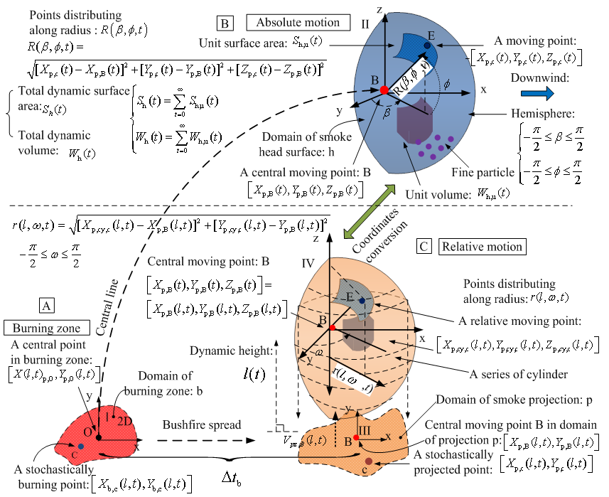Figure 1. (A) temporal and spatial diffusion of smoke plume over burning zone; (B) hemispherical model for determining stochastic diffusion of smoke plume and relevant properties; (C) cylindrical model for calculating horizontal displacement of particles and correlating them with elevation

The absolute and relative displacements of smoke particle are easier expressed in the horizontal plain than in the vertical. For the currently moving positions, a set of points [X_p,c(t) , Y_p,c (t)] (see Figure 1(B)) are determined by both the spatial position of centre of mass point B [X_p,B(l,t) , Y_p,B (l,t)] and the diffusion positions [X_p,cy,c (l,t), Y_p,cy,c (l,t)] relative to point B in the coordinates IV (see Figure 1(C)). They are described by equations (1)−(2) respectively. However, the current temporal and spatial position Z_p,c (t) in equation (3) is discussed separately because of its special characters.

Where, the point [X_p,B(l,t) Y_p,B(l,t)] are assessed by two sets of equations (4)−(5).

(4)

(5)

Where,

(6)

Several attentions should be drawn to equation (1)−(6) are those.

1. To obtain [X_p,c(t) , Y_p,c (t)] of particles in coordinates II and effectively correlate them with the corresponding elevations as well, the approach relies on the coordinates conversion between coordinates II and IV. Thus the term XC and YC at the right side of equation (1) and (2) is obtained through the coordinates IV respectively.

2. A set of [X_p,c(t), Y_p,c (t)] is a group of absolute horizontal position of particle in coordinates II, each of their spatial positions fail to be determined by itself. A set of [X_p,cy,c (l,t), Y_p,cy,c (l,t)] is a group of relative horizontal positions of particles in coordinates IV. They are not only moving with time t but also described by dynamic height l, which is much convenient to establish relationship with DEM in the coordinates IV. In order to determine the horizontal position of each particle, the same size [X_p,B(l,t) , Y_p,B (l,t)] must be added into [X_p,cy,c (l,t), Y_p,cy,c (l,t)].

3. Both of[X_p,c(t) , Y_p,c (t)] and [X_p,cy,c (l,t), Y_p,cy,c (l,t)] represent the same particles at current time (denoted by c) projected onto the same domain p. However, in order to distinguish them, an extra subscript cy (which denotes cylindrical coordinates) is added into terms Such a separate treatment is convenient for modelling.

4. As seen from equation (1)−(2) and (4)−(5), the horizontal displacement of particles in smoke plume along x and y direction is influenced by local geostrophic wind which is only confined within the domain b or p. Its magnitude is affected by its dynamic height l. Because it is a dynamical process, it is also changed with respect to the elapsed time t. Consequently, both l and t as parameters are considered into the horizontal displacement to show correlation with local geostrophic wind.

5. [X_p,B(l,t) , Y_p,B (l,t)] indicates that the same size points of center of mass in horizontal direction are also affected by corresponding l and t.

6. The velocity of geostrophic wind V_p,O (l,t) originating from the point O to be changed in the domain p in one time interval Δt_b is used for calculating smoke plume displacement of one center of mass B shown in equations (4)−(5).

7. The V_,O (l,t) can be derived and estimated from equation(7).

(7)

Where, Max (:) is a built-in function in MATLAB^® (similarly for others except indicated in this paper) to generate maximum value. The V_geo,O (l,t) is velocity of geostrophic wind at the location O (see Figure 1(C)). The ε(l) is a dimensionless ratio of V_act,geo to V_geo, which was introduced in part 1. The reason why the maximum value is selected is that the point O could be located at a large scale burning zone with different elevations and the velocity of actual geostrophic wind is also changed with respect to the dynamic height l of smoke plume and time t. To easily consider the variety of geostrophic wind, the ε(l) is used here.

8. The point [X_b,O (l,t), Y_b,O(l,t)] represents that whose dynamic position is specified by the point O at the centre of mass in the burning zone. A set of burning spots is moving forwards downwind.

9. As seen, the x and y horizontal displacement of smoke plume from point O to the current point B (thus from [X_b,O(l,t) , Y_b,O (l,t)] to [X_p,B(l,t) , Y_p,B (l,t)] downwind) is influenced by the resolved velocity of geostrophic wind V_geo ( thus V_px,O (l,t) and V_py,O) and its elevation, angle α ,azimuth θ within the burning time interval Δt_b. The subscript px and py represents that the velocity of geostrophic wind is resolved into two components and projected onto domain p in x and y direction respectively. τ(t) is a dynamic horizonatal diffusion coefficent introduced in part1to mathmatically illustrate how displacement of horizonatal diffusion is affected by the velocity of smoke mixture.

10. Usually, which is caused by the relative velocity of airflow to the velocity of earth rotation, however the elevation angle β relies on how fast the smoke rises from ground, which is affected by many forces at the initial time. Therefore, in general, the angle of from 25° to 90° at ground level and changes to approach to α at high level.

At this stage, X_p,B(l,t) and Y_p,B (l,t) used in the equation (1) and (2) are determined. Other parameters are confirmed by building two models being discussed in the following sections.

2.2. Account for Self Temporal-spatial Dispersion of Smoke Plume by Means of Models

In practice, the most important in investigating the spatial behaviour of smoke plume is to assess how the particles in smoke mixture with different velocities relative to one center of mass disperse in multi-direction. The concept of conversion of coordinates was introduced in part 1 and briefly applied into calculating the horizontal displacement of smoke plume in the last section. In this section, the conversion of coordinates is further illustrated by building two coordinates-based models used to describe the displacement of particles especially in vertical direction and solving the problem raised from calculating the horizontal displacement of particles of smoke plume in equation (1) and (2).

A. Hemispherical Model

As mentioned in part1, for the spatial diffusion of smoke, the particles radially disperse in plain y-z plain in the coordinates II (see Figure 1(B)) and presents normal distribution. The hemispherical model especially focuses on the head of smoke plume. However, the dispersion of smoke in x-y plain is thought of as carrying out along direction of Z. Due to downwind, the diffusion happens in other side hemisphere along x direction can be ignored. That is why it is named as a hemispherical model.

Some main features about hemispherical model are emphasized as follows.

1. The distribution of particles in the hemispherical model is stochastic.

2. The main advantage of the hemispherical model is that the shape supplied by this model is approximate to the real case of smoke plume and calculating physical properties such as volume, radius and surface area of head of smoke plume is easily performed. The detailed performance in this field is to be implemented later.

3. The spatial position of each stochastically distributed particle has corresponding elevation with respect to elapsed time in the domain of smoke plume projection.

4. The main drawback for hemispherical model is that it fails to establish the direct relationship between the vertical displacement of particles and their corresponding elevations owing to lack of information about radius for each particle.

Consequently, the advantages that the hemispherical model owns are remained and its drawbacks are to be solved by cylindrical model by means of the conversion of coordinates.

B. Cylindrical Model

Consider above factors in the hemispherical model, all features which particles have are cloned to be handled in a cylindrical coordinates thus the coordinates IV (see Figure 1 (C)).

The expansion of smoke volume in the coordinates IV can be considered as the horizontal displacement of a group of particles along with z axis. However, in practice the following factors are helpful to model the physical behaviours of particles in comparison with the case in the coordinates II.

1. The particles located on hemispherical surface in the coordinates II are described and located on a number of cylinders with different radius in the coordinates IV.

2. In the coordinates IV, the pattern of particles diffusion is radial and around the z-axis where the origin B is located. The point B is treated as a relative stationary point in this case. The radius used in depicting particles is r(l,ω,t), which varies with Z_p,cy,c(t) (see Figure 1 (C)). Where, ω can range between –π/2 and π∕2 to respond to the hemispherical model or −π and π to the sphere. In contrast with the case shown in the coordinates II, the dynamic radius r(l,ω,t) points from the arbitrary point along with the z-axis to an arbitrary point (e.g. point E) on a unit surface .

3. The volume occupied by particles in the coordinates IV can be thought of as its volume being stochastically expanded from its initial state in the burning zone with respect to time t.

Therefore, a set of points [X_p,cy,c (l,t), Y_p,cy,c (l,t)] in x-y plain in the coordinates IV can be assessed by equation (8)−(9).

(8)

(9)

As to the terms in equation (8) and(9), they are explained as follows.

1. The term XE and YE is a dynamic displacement in x and y direction respectively, which commences from the point O in burning zone (see Figure 1(A)) at the initial time t_i (the subscript i denotes initial time). In this case, the initial time t_i is used to emphasize on counting the time of smoke plume ascending from ground. However physically speaking, the smoke plume is invisible when the elapsed time t=0. In other words, the elapsed time t must be larger than zero thus t >0 when the smoke plume become visible. In order to conveniently calculate, the elapsed time t shown in all equations in the context is actually counted from t_i=0 as a starting point of time and assuming smoke plume is visible. Therefore, the subscript i is dropped in the calculation.

2. The term XE and YE is individually treated as an increasing unit magnitude within the time interval Δt_b. It can also be interpreted as the effect of self-diffusion of smoke plume on the displacement in x and y direction when its volume consisting of massive unit volumes (see Figure 1(A)) is spatially expanding with respect to the elapsed time t.

3. Assume that the stochastic distribution of particles is performed as a normal distribution; therefore it is expressed by a series of random number which is generated from the built-in function Randn(n,m), where n=1 to constitute a set of spatial points of particles appears in the coordinates IV (see Figure 1 (C)) in one direction.

4. Consider the scale of diffusion is developed from the original state, accordingly, unity is added into the term XA and YA respectively.

5. The term XD and YD is generated by multiplying the term XE and YE with the term XA and YA respectively. The implicit physical meaning is that the volume of smoke plume is increased with respect to the elapsed time t remaining the original scale.

6. is a dynamic self-diffusion coefficent which was introduced in part 1. In this case, it implicitly how the viscosity of smoke plume affects the displacement in x and y direction.

Up to this point, the points [X_p,c(t), Y_p,c(t)] shown in equation (1)−(2) are able to be confirmed by combining equations (4)−(7) with equations (8)−(9). In the following sections, the vertical displacement of particles is to be considered.

2.3. Determine Temporal and Spatial Location in Vertical Direction

Once the points [X_p,c(t),Y_p,c (t)] in smoke plume is confirmed, Z_p,c (t) in equation (3) is considered now. The first term H_p,c (t) shown at right hand of the equation (3) can be processed by equation(10).

(10)

Where

The Demf (:,:) is a function linking the horizontal positions in a plain coordinates to the corresponding elevations where the particles in smoke plume are projected onto, which is created in terms of the conversion of vector point in the coordinates of DEM and principle of linear indexing respectively introduced by author[14].

Hence, the elevation of particles H_p,c (t) in the domain p of landscape is determined by a set of horizontal points [X_p,c(t),Y_p,c (t)].

The remaining problem is how to assess the vertical displacement of particles in the coordinates IV: Z_p,cy,c(l,t), which can be assessed by equation(11).

(11)

Where

(12)

Similarly, several issues related to equation (11) and (12) need to account for as follows.

1. The V_pz,B (l,t) in the term ZV can be thought of as a series of velocities of particles rising from the ground (thus the domain p) and vertically distributing around z-axis where center of mass B is located in the coordinates IV.

2. Although the distribution of velocities is influenced by the many forces during the time interval of smoke plume rising from ground, the effect from those forces is considered by a vertical dynamic diffusion coefficient λ(t), which was introduced in part1.This dynamic coefficient is integrated with the vertical component velocity of local geostrophic wind V_pz,_B(l,t), which is obtained by the equation (12).

3. The term V_p,_B(l,t) represents the velocities of geostrophic wind at the point B within the domain p in with respect to dynamic height l (see Figure 1(C)).

4. The distribution of vertical displacement for each particle is stochastic. This approach can be expressed by multiplying the term ZV with a set of random numbers (between zero and one) generated by term ZD within the time interval Δt_b.

5. The built-in function size (:) generates a scale of projection area with the same size as H_p,c (t).Thus, in other words, each particle in smoke plume is stochastically projected into the domain p.

6. If one of heights Z_p,cy,_c (l,t) approaches to zero, it means one particle approaches to or deposits onto the ground, otherwise it moves towards sky.

At this stage, the temporal-spatial positions of particles diffusion in each sub-volume of smoke plume associated with [X_p,c(t), Y_p,c(t), Z_p,c(t)] shown in equation (1)−(3) is already determined. The correlation between smoke plume in the sky and burning zone on the ground, corresponding elevations is also achieved.

In the following sections, the concentration is moved onto seeking the center of mass for smoke plume so as to calculate some physical properties of smoke plume.

2.4. Position Temporal and Spatial Center of Mass for Smoke Plume

As mentioned previously, although the direction of spatial dispersion of smoke plume at the horizontal level can be determined by either the angle between burning and smouldering zone or measurement, determining the spatial location of center of mass for each sub-volume of smoke plume in vertical direction still relies on the stochastic distribution of particles.

The temporal-spatial location for any center of mass in horizontal plain can be determined by equations (4)−(5). However, strictly speaking, the distribution of particles is uneven especially at lower ground level, which is directly influenced by the terrain. The best way to handle it is to choose the mean of vertical displacement of particles in the coordinates IV. Therefore, the location in vertical direction can be positioned by using equation(13).

(13)

Where

(14)

In this case,

1. The dynamic height of center of mass Z_p,B (l,t) on the central line is decided by two the terms. Thus the elevation H_p,B (t) and the average dynamic height of particles disturbed in the sub-volume of smoke plume centred by the point B within domain p.

2. The average dynamic height shown by term ZE indicates that the center of mass B in vertical direction is located at a middle point where the bidirectional dispersion of smoke mixture can maximally reach to (see Figure 1 (C)). However, the point B is remained in the central line downwind.

3. Both Max (:) and Min (:) are built-in functions to find maximum and minimum value.

4. The elevation H_p,B (t) can be obtained by the point [X_p,B(l,t) Y_p,B(l,t)] which is able to be confirmed by equation (4) and (5) through the function: Demf.

5. In terms of (13) and (14), the points of the center of mass consisting of the central line waves up and down forwards and are also affected by the corresponding elevation of terrain.

At this stage, the spatial position of center of mass located in each sub-volume of smoke plume is determined. In the rest section, the manner of calculating physical properties of smoke plume is to be decided.

2.5. Estimate Surface Area and Volume of Smoke Plume Front

In the last section, the spatial position of particles in smoke plume produced by the equation (1) and (2) is already determined. However, investigating the physical properties such as volume and surface area of smoke plume are also concerned in modelling.

To estimate the surface area and volume of each dynamic smoke plume head, it should return to the coordinates II.

In theory, from the micro analysis, the enlargement of dynamic volume of smoke plume head W_h (t) can be explained as a process of infinitely accumulating a number of small volume elements W_h,u(t) (the subscript h,u denotes head and unit respectively)with respect to a dynamically increasing radius. The original size of smoke volume is remained. Similarly, the total dynamic surface area of smoke plume head S_h (t) is the sum of the unit surface S_h,u(t) with respect to time (see Figure 1 (B)). The relationship can be shown by equation(15).

(15)

The micro analysis is useful for further investigation. However, in this research, the attention is restricted to calculate the geometric quantity of the smoke plume head during its temporal-spatial dispersion.

In calculating W_h (t) and S_h (t), both of them can be estimated by combining the point of center of mass (X_p,B(l,t),Y_p,B(l,t), Z_p,B(l,t)) and a series of stochastic points (X_p,c(l,t), Y_p,c(l,t), Z_p,c(l,t)). In this case, the volume where the point B is located is assumed as a head of smoke plume, the same treatment is also applied into other center of mass in each sub-volume during the calculation.

For a ‘top hat’ like head of smoke plume, its dynamic radius can be approximately calculated by equation (16) and the point B is chosen as a central point of the hemisphere and the origin in the coordinates II. In order to simplify the expression of equation, the dynamic height l is dropped in the context of this section.

(16)

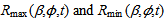
It can be discovered that massive radii exist in the hemisphere and are distributed stochastically. An effective manner is to find out dynamic maximum and minimum radius using equation (17)−(18) at first and then apply an average radius into equation (19) −(20) to obtain S_h (t) and W_h (t). The subscript max and min indicate maximum and minimum value.

(17)

(18)

(19)

(20)

Up to now, the manner of assessing the surface area and volume of smoke plume is already decided. The results of modelling in virtue of previously established models and equations are to be displayed and analysed in the next sections.

3. Modeling Conditions

3.1. Select Geographical Location for Modelling

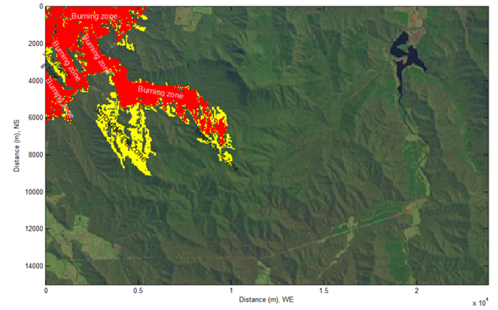Figure 2. classified burning and smouldering zone at a selected geographical location shown in the remote sensing imagery

Modelling the large scale temporal-spatial dispersion of smoke plume is based on the place where bushfire often took place historically in Victoria, Australia. The geographical location (-36°70'10" S, 146°44'30" E; -36°83'60" S, 146°71'00" E) is shown by Figure 2. The feature of terrain and distribution of vegetation is stored in the remote sensing imagery captured by the satellite LANDSAT. The corresponding DEM is shown by Figure 3.

3.2. Select One Burning Spot from a Classified Burning Zone

The burning zone and smouldering zone was already classified at two different places based on the sequence of bushfire spread in the given digital imagery using the technique in the digital image processing in terms of the difference of grey level for each colour component stored in the remote sensing imagery at the beginning of modelling[14] (see Figure 2). The geographic location and distribution of vegetation is then transferred into the corresponding DEM (see Figure 3) by means of the technique of indexing.

3.3. Initial Geometric and Physical Properties at Burning Zone for Modelling

The area of original burning zone is 3.4217e+005 m² and the area for currently burning zone is 2.8175e+006 m². The center of mass in the currently burning zone[X_p,O(l,t) , Y_p,O(l,t), Z_p,O(l,t)] is (5.6778e+003 m, 1.9752e+003m, 397.7040m) at dynamic height l = 397.7040m and time t = 0. The maximum distance of a stochastic burning spot from the center of mass located in the currently burning zone {Max[X_b,c(t)], Max[Y_b,c(t)]} is (6.6835e+003m, 2.8557e+003m) at time t =0. Then, the radius of smoke plume R(β,𝜙,t) at the initial time t_i is 1.3367e+003m.

Above data can be obtained by calculation integrating DEM with the remote sensing imagery and linear indexing technique.

Accordingly, it is assumed that the bushfire spread happened on the ground and smoke plume rose from the currently burning zone at the same time before start to model the temporal-spatial dispersion of smoke plume. Furthermore, the direction of smoke plume downwind is determined by the angle between the burning and smouldering zone. The angle is 74.8580° clockwise in this case. In reality, this angle can be determined by a measured wind direction.

4. Results Visualization and Discussion

4.1. Results Visualization

Several data with specific properties are calculated and obtained by means of above proposed models with respect to the elapsed time t. The results of them are visualized in Figure 3−Figure 5 respectively.

4.2. Analysis of Phenomena and Discussion

The results shown in Figure 3−Figure 5 also contains some physical properties; they are displayed in Figure 6−Figure 8 respectively.

A. The influence of terrain on the smoke plume

According to Figure 3−Figure 5 and the case (A) and (B) in Figure 6−Figure 8, it can be also found a fact that the properties of smoke plume varies with the feature of terrain at the ground level. They change with respect to the geometric features of terrain such as height and slope. The phenomena are those

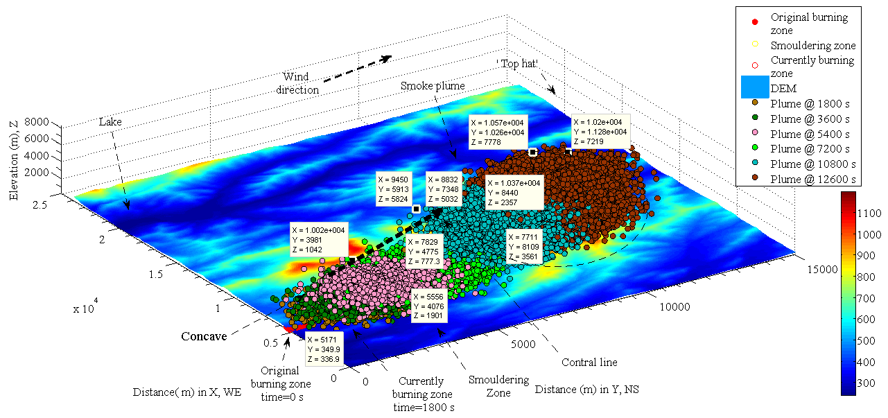
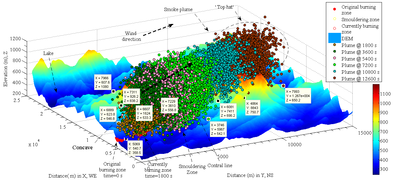Figure 3. temporal and spatial dispersion of smoke plume in landscape with respect to elapsed time (side view)

Figure 4. temporal and spatial dispersion of smoke plume in landscape (top view)

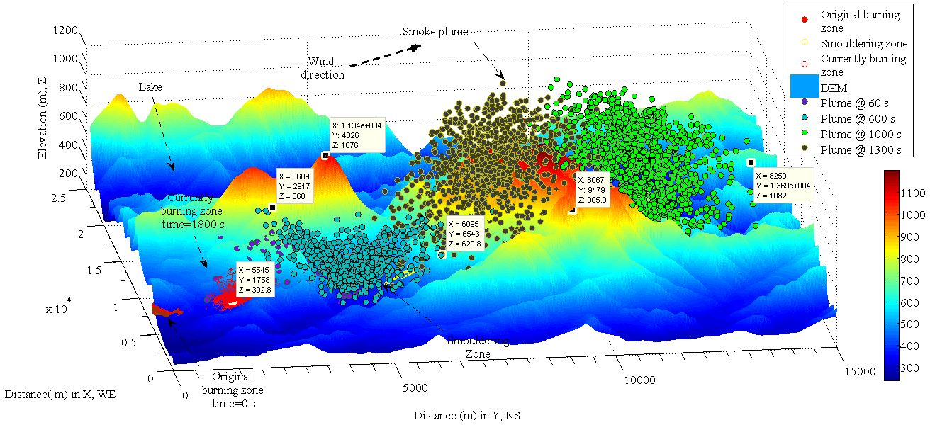Figure 5. temporal and spatial dispersion of smoke plume in landscape (a large dynamic diffusion coefficient)

1. The heavy smoke is remained in the valley

That is because, in reality, in terms of the theory of fluid dynamics, the turbulence of air at a valley is always formed when air has different velocity at different layer (height). The horizontal velocity of smoke plume in Figure 5 is much faster than that in vertical direction due to influence of geostrophic wind. Therefore, a certain amount of smoke is remained in the valley; it is very similar to the case of Maxwell−Stefan mass diffusion. The vertical diffusion velocity of this part of smoke relies on the horizontal velocity of geostrophic wind at top of hill.

2. The smoke plume flows faster uphill than downhill at ground level

Such a phenomenon is similar to the bushfire spread at ground[15]. The velocity of air fluid is accelerated because the vertical component of velocity of geostrophic wind is increased with respect to the height of hill.

Above two points are useful information for fire fighters and local residents who want to escape from the burning zone in an emergency.

B. The impact of geostrophic wind on the smoke plume

1. The dynamic height and horizontal displacement of each smoke plume is increased with respect to the elapsed time t (see Figure 3 and Figure 6 (A)).

With the ascent of smoke plume, the magnitude and direction of geostrophic wind is dramatically increased and moderately altered respectively. Also the front of smoke plume obviously forms a ‘top hat’-like head and a ‘concave’ appears implicitly and distributes along the top of smoke plume downwind because of the viscosity of smoke mixture and high speed of geostrophic wind at high level (see Figure 3 and Figure 4).

In reality, the viscosity of smoke mixture is not constant. The diverse dynamic diffusion coefficients are then introduced into modelling to approach to the real case and illustrate some phenomena were discovered.

2. The maximum and minimum dynamic radius of each front head of smoke plume is in general increased with respect to the elapsed time t respectively (see Figure 3 and Figure 7(A) and (B)). The maximum height of particle in smoke plume may be able to reach to 8000 meters in about 3.5 hours later if the vertical diffusion of smoke plume follows up the geostrophic wind.

3. Similarly, the dynamic surface area S_h (t) and its volume W_h (t) of smoke plume are dramatically increasing with respect to the elapsed time t (see Figure 8(A) and (B)).

As seen, all properties of smoke plume are greatly influenced by the geostrophic wind. There are several steps of altering the velocity of geostrophic wind with respect to height. At ground level thus the height is less than 1000 meters, the frictional force plays a main role in resisting against the acceleration of the geostrophic wind. However, the geostrophic wind starts to increase from 1000 to 1400 meters height due to the less effect from the top of mountain on it. When the height is between 1400 and 3000 meters, the main frictional force is generated by air. When the height is over 3000 meter, the frictional force is negligible, the velocity of geostrophic wind increases dramatically (see Figure 6 (A) and (B)). It can be concluded that the velocity of geostrophic wind at the top of smoke plume is always larger than the one at the central level and ground level thus V_geo,top > V_geo,center > V_geo,ground.

C. The effect of dynamic diffusion coefficient on the smoke plume

The effect of dynamic diffusion coefficient on absolute and relative displacement of particles is obvious.

As motioned above, the difference between Figure 3 and Figure 5 is caused by using different horizontal diffusion coefficient in x and y direction in comparison with the case in Figure 3.

The dynamic diffusion coefficient used in Figure 5 is about 100 times as large as the one used in Figure 3. That results in that the smoke plume is quickly dispersed. The dynamic diffusion coefficient can represent the physical feature of heavy or light smoke produced y burning different vegetation. They are adjustable according to the measurement of local actual wind. In contrast, because of such a unique character appearing in modelling, forecasting the spatial dispersion of smoke plume become possible on the basis of calculating the local velocity of geostrophic wind and adjusting the dynamic diffusion coefficients.

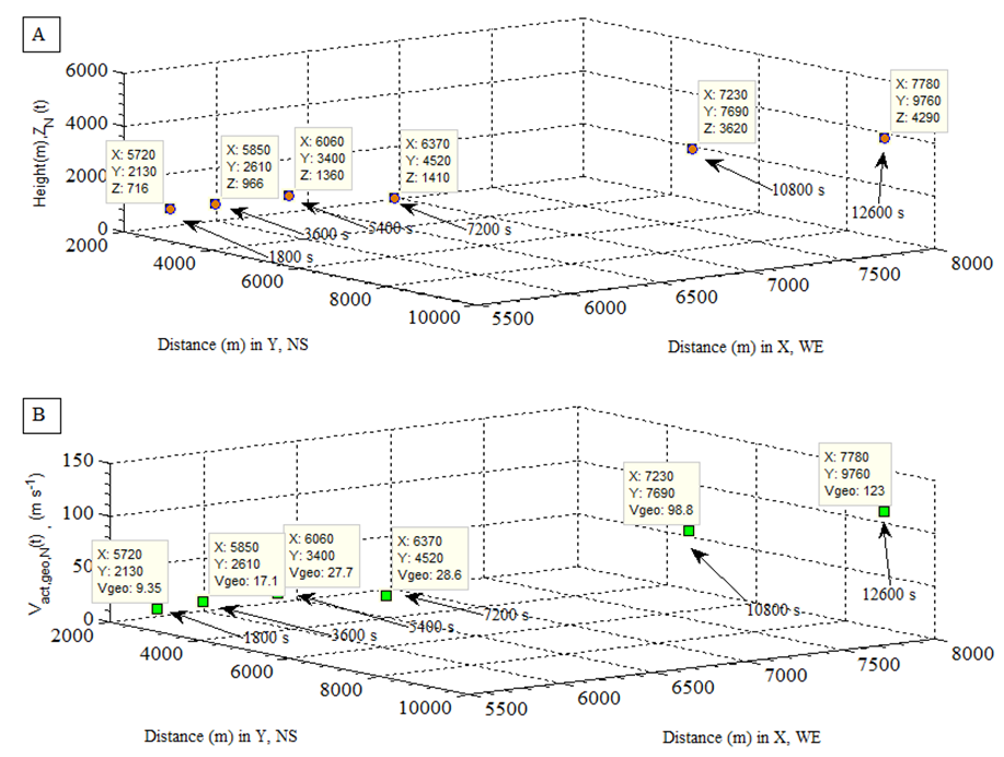Figure 6. (A) dynamic height of center of mass of smoke plume; (B) actual velocity of geostrophic wind at each center of mass with respect to elapsed time

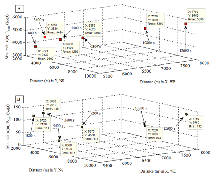Figure 7. (A) dynamic maximum radius of smoke plume head; (B) dynamic minimum radius of smoke plume head

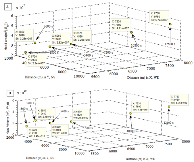Figure 8. (A) dynamic head surface of smoke plume; (B) dynamic head volume of smoke plume

Figure 9. display bushfire and smoke plume in satellite imagery (top view)

4.3. Compare Results of Modelling with Real Historical Bushfire

The remote sensing imagery shown in Figure 10 captured the real situation of bushfire spread and the dispersion of smoke plume happened at Victoria, Australia in 2006 at the same geographic location. It can be seen that the spatial location and direction of smoke plume varied with time, direction and velocity of geostrophic wind.

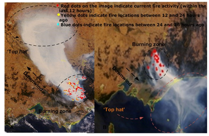Figure 10. historical bushfire with a large scale dispersion of smoke plume took place in Victoria, Australia 2006[16]

In addition to general case, the unique character of smoke plume appeared in Figure 10 at high level is that

1. The ‘top hat’-like front of smoke plume became larger and larger with respect to the elapsed time.

2. The ‘concave’ appeared at the top of smoke plume and closed to its head.

3. The amount of surface area and volume is increased markedly.

4. Consequently, the concentration of smoke plume decreased at high level. Although the remote sensing imagery failed to supply the height of smoke plume because it was captured by the satellite from its top at about 100 km height, it at least reached to over 3000 meters vertically. This figure is estimated by the small scale bushfire experiment [17]. Then the smoke plume thus its front head was invisible, because its concentration was completely diluted in a few hours. However, above situation was a static description, for a large scale smoke plume could maintain many days under the weather condition of bushfire.

A. Similarity

The results gained from the simulation satisfactorily meet the scenario of bushfire captured by satellite. Figure 4 in the modelling is viewed from the top. Therefore, drawing a comparison between Figure 4 and Figure 10 yields that

1. Both of them have a ‘top hat’.

2. Their trajectories are shown as a parabola.

B. Difference

The main geometric difference is that the concave in modelling is implicitly appeared by the measurement (see Figure 3 and Figure 4 ).

It is difficult to point out more differences in terms of the results generated by using two different manners. However, the modelling has much unique functionality which the remote sensing imagery is unable to have.

Based on modelling, it is able to

1. Calculate the velocity of geostrophic wind and decide its direction and estimate how much it affects the dispersion of smoke plume.

2. Integrate with the progress of bushfire spread on the ground.

3. Assess how the geometric features of terrain affect the dispersion of smoke plume on the ground.

4. Estimate some geometric parameters such as radius, volume and surface area for smoke plume.

5. Forecast the temporal-spatial dispersion of smoke plume.

6. Display its 3D results in the corresponding 2D remote sensing imagery.

4.4. Display 3D Modelling Results in Satellite Imagery

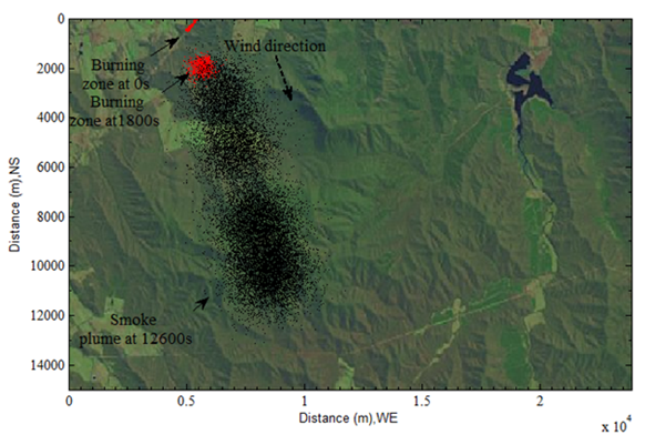
This is an extra topic in discussing results from modelling.

Sometimes, in order to clearly visulize and verify the results of three-dimensional modelling in the different view, they are able to be transferred into two-dimensional satillite imagery on the basis of the technique of lenear indexing. The bushfire spots, temporal and spatial dispersion of smoke plume shown in Figure 3 are accurately transferred into the satillite imagery in Figure 2 and displayed clearly. During the transfer, data of bushfire and smoke plume are store into a datebase respectively. As seen from Figure 9, the bushfire and smoke plume generated by modelling are completely “melten” into the original remote sensing imagery. It is much esier to examine the results of modelling under the real background.

5. Conclusions

Modelling the temporal and spatial dispersion of smoke plume in the frame of DEM is a complicated process; it requires multidisciplinary knowledge including some creative techniques. This complicated process has been classified into several sub-processes. They occur individually and simultaneously and are also correlated mutually. The proposed resolutions to the initial objectives of this research have emerged in such complicated correlations although they have been resolved individually.

A. Summary of current work

The detailed process of modelling and explanation has already been performed previously. The main correlation as conclusions for the current work is summarized as follows.

1. The dispersion of smoke plume including bushfire spread is a dynamic process. The elapsed time is counted from one point of the continuous time sequence based on the one specific location of bushfire spread when the smoke plume is visible initially. Defining the elapsed time for a specific process is for easily interpreting some phenomena. Accordingly, the time interval is used to count how much time it is consumed to finish one certain process and then account for how fast it is. No matter where the processes take place, all of them happen simultaneously.

2. The smoke plume is elements manually partitioned into a series of instantaneous volume. Such a treatment is purely for easily simplifying the case. In real life, for light smoke plume, such phenomenon does exist.

3. The central line is formed by a number of center of mass moving up and down along it. In fact, the center of mass cited from physics and used for each sub-volume element of smoke plume is unmeasurable. However, the concept of center of mass in this modelling is only used for explaining some physical phenomena. No matter how to explain the central line, it can be assumed that the central line exists because the dispersion of smoke plume always happens downwind.

4. A series of the spatial position of center of mass of smoke plume contains the corresponding variation of the physical and geographic properties held by sub-volume elements with respect to the time. Such a process simultaneously happens accompanying with bushfire spread on the ground.

5. No matter how big size the substance in smoke mixture is, the smoke (molecule size) and granule (visible size) are treated as particles so as to easily model in this research.

6. The same observed objects such as particles can be traced and described in the different coordinates. Thus, the desired physical properties of the observed objects can be obtained by means of building different coordinates.

7. In the research, the velocity and displacement of particles can be classified into the absolute and relative in virtue of physics. It is one of most difficult topics to be determined. The conversion of coordinates is then used, which plays a significant role in the process of acquiring diverse physical and geometric properties held by smoke plume. The advantage of conversion of coordinates is that the real spatial position of the same observed object (or particle) is not altered during conversion of coordinates. However, the desired properties can be easily achieved. Such a treatment is very similar to often used Laplace transform in mathematics.

8. The absolute displacement of particles is acquired by transferring the particles into other coordinates and assuming burning spot on the ground as stationary observed spot.

9. Individually finding spatial location correlating with the corresponding elevation for each particle is another difficult topic. However, the conversion of coordinates is also able to successfully solve the difficulties.

10. Specifying domain is a useful manner of focusing on specific case concerned about. Several specific domains were created in modelling. The domain on terrain formed and projected by each sub-volume of smoke plume is always considered through the modelling. Such a domain not only helps to find out how the spatial particles distribute but also establish the relationship of with their elevations associated with DEM. This domain is often combined with the cylindrical coordinates-based model in determining spatial position of particles in vertical direction.

11. Choosing the appropriate manner of stochastic distribution for particles is one of important issues in the modelling. The normal distribution of particles is used to describe how the particles position spatially along the central line in the horizontal plain downwind. It could be fairly reasonable according to the observation from the remote sensing imagery. However, such a treatment is not suitable for stochastic distribution of particles in the vertical direction. Consequently, the standard uniform distribution is adopted to ensure the particles either ascend from the ground or descend to deposit on the ground.

12. Modelling smoke plume has to rely on one important natural phenomenon hence the geostrophic wind. It plays a prominent role in prompting the diffusion of smoke mixture spatially.

13. The formation of geostrophic wind is caused by several forces. Its velocity is able to be resolved into horizontal and vertical component. Those components vary with increasing elevation. It is difficult to directly measure how much the diffusion of smoke plume is affected meanwhile. Accordingly, introducing appropriate dimensionless dynamic diffusion coefficients is quite necessary. Furthermore, the ratio of actual geostrophic wind and geostrophic wind is also introduced and involved in the dynamic calculation of geostrophic wind for the sake of convenience.

14. Another important concept which is introduced about the coefficient is a dynamic self-diffusion coefficent. Except for the absolute motion of particles, the relative motion appears in the form of self-diffusion. In reality, the process of self-difffusion is resisted by the friction force between diffused gasous mixture and ambient air thus kinematic viscosity of smoke plume.The dynamic self-diffusion coefficent is also a dimessionless dynamic coefficient.

15. In the process of positioning self-diffused particles, the dynamic height was introduced. It helps to establish the correlation amongst elevation of terrain, that of geostrophic wind and spatial displacement of particles.

B. Future work

On the basis of the current work, the achievement has provided several opportunities for further research. In reality, the smoke plume is a main factor in poisoning resident and fire fighters, impacting on environment and especially in forming the smouldering zone. Substantially, the smoke plume is not only a kind of pollutant but also an energy carrier. The released energy from it in the form of radiation is a big source to heat the remote vegetation and then accelerate bushfire spread on the ground.

In this research, each sub-volume has temporal-spatial properties. They can be associated with the geographic, meteorological properties as well as the heat, mass transfer. Those potential correlations will be able to estimate:

1. What an amount of smoke pollutant is to be dropped onto the ground downwind.

2. How the carried energy in smoke plume impacts environment.

3. How big area of smouldering zone is formed before the bushfire arrives in.

Those approaches will play a considerable important role in forecasting bushfire spread and providing useful information for resident and fire fighters.

ACKNOWLEDGENTS

Author wants to offer special thanks to Professor Jing. X. Zhao at Shanghai Jiao Tong University for supplying desired data used in this research.