Carl Y. H. Jiang
Centre for Intelligent Systems Research, Deakin University, Victoria, 3216, Australia
Correspondence to: Carl Y. H. Jiang, Centre for Intelligent Systems Research, Deakin University, Victoria, 3216, Australia.
| Email: |  |
Copyright © 2012 Scientific & Academic Publishing. All Rights Reserved.
Abstract
Smoke Plume is a pollutant produced by large scale bushfire. However, effectively modelling a large scale dispersion of smoke plume has not been reported. In this research, a novel method has been proposed. Modelling is based on Digital Elevation Model integrating with meteorological parameter. The smoke plume is treated as massive fine particles. Their absolute and relative motions over landscape are determined by setting up different spatial coordinates. In order to establish the correlation between their spatial positions and elevation of digital elevation model, several new concepts have been introduced. Smoke plume is portioned into a series of sub-volume locating on the dynamic center of mass. The concept of domain not only confines the region of smoke plume projected onto the surface of terrain correlating it with elevation but also describes the spread of bushfire on the ground and details spatial diffusion of smoke plume. The elapsed time is also redefined according to specific physical meaning to illustrate how smoke plume disperse simultaneously accompanying with bushfire spread. Several proposed delay coefficients is used to consider the viscosity of smoke plume and describe how fast smoke plume disperses in three-dimensional space. Obtaining physical properties of smoke plume is achieved by conversion of coordinates. The technique of linear indexing is fully applied into all processes occurring in bushfire spread and accurately control them in the process of data and information transfer. Modelling has been classified into two parts. In the part1, the focuses are on explaining some introduced concepts in detail.
Keywords:
Smoke Plume Modelling, Digital Elevation Model, Spatial Dispersion, Smoke Plume, Bushfire
Cite this paper: Carl Y. H. Jiang, Modeling Temporal and Spatial Dispersion of Smoke Plume Based on Digital Elevation Model (Part 1), American Journal of Geographic Information System, Vol. 2 No. 4, 2013, pp. 82-92. doi: 10.5923/j.ajgis.20130204.02.
1. Introduction
The smoke is a product generated by burning vegetation in landscapes. The smoke plume is downwind formed by molecules diffusion in sky accompanying with bushfire spread, which is a gaseous mixture consisting of molecules and a series of different size and shape fine granule or soot. The molecules can be CO2, SO2, NO2 and NO, etc. depending on the sort of vegetation is being burnt[1]. However, the carbon dioxide is main component of gaseous mixture, which is gray gas. Of importance is that the gray gas and soot are capable of carrying and radiating energy[2, 3].It dramatically affected on the smouldering zone[4]. Therefore, investigating smoke plume is helpful and valuable in forecasting bushfire spread and providing useful information for resident and fire fighters. Although the various properties of smoke plume have been investigated by many researchers for many decades [5-10], and some researchers have even tried to detect some physical and thermal properties for large scale smoke plume and bushfire spread such as the distribution of concentration of smoke burning temperature by means of satellite imagery and lidar experiments respectively and attempted to model smoke from forest fire[11, 12].A very clear fact is that it is impossible to obtain the relevant information by means of experiments and technique of remote sensing so as to quantitatively and effectively estimate and forecast large scale three-dimensional smoke plume produced by bushfire. Accordingly, a novel method of investigation in this field is to be proposed in this research and introduced as follows.
1.1. Features of Research
1). the new approach is based on DEM.A group of parameterized models integrating with geostrophic wind, digital elevation model (DEM) and stochastic processes is to be built and analysed. This is an important step to discover the potential relation between bushfire spread on ground and temporal spatial dispersion of smoke and then find out the geometric properties of smoke plume.2). The molecules and fine particles are treated as points.Although the amount of molecules and fine particles has their own intensive and extensive properties in their physicochemical aspects respectively, they are not to be taken into account in this paper.
1.2. Objectives and Scope of Research
The research in the field of modelling the temporal-spatial dispersion of smoke plume is to explore the following topics:1). How the smoke plume is physically treated.2). Why the elapsed time is redefined and how it is used in describing each dynamic process in detail.3). Why and how the motion of particles in smoke plume is classified.4). How several coordinates and domains used for modelling the process of smoke plume dispersion and bushfire spread are built and defined.5). what the functionalities of domains are in dealing with dynamic processes.6). How the geostrophic wind is formed and involved in modelling large scale smoke plume. 7). what the relationship between the temporal-spatial positions of particles in smoke plume and DEM are. How they are correlated with DEM by means of the conversion of coordinates to calculate displacement.8). Why the dynamic diffusion coefficients, height and ratio of geostrophic wind are introduced. How they are applied.9). How the velocities of particles in smoke plume are estimated. How the self-diffusion of smoke plume is described and modelled.10). How the behaviours of smoke plume are integrated with those of bushfire spread. 11). How the specific model is used to estimate geometric scale of smoke plume head.Meanwhile, a hemispherical model combining with a cylindrical model for spatial diffusion with stochastic approach is to be proposed and discussed. Eventually, the result of modelling is to be compared with the historical large scale smoke plume captured by the satellite imagery at the same geographic location. However, in order to detail each procedure of modelling. The research has been portioned into two parts. In the part 1, the scope is focusing on some terms and definitions correlated with the modelling. The results and their analysis are to be implemented in the part 2.
2. Methodology
As well known, bushfire spread is a very complicated process, consequently modelling the process of combining the temporal-spatial dispersion of smoke plume with bushfire spread in landscape requires many specific terms and detailed illustrations. In the following process of defining and interpreting them, the multidisciplinary concepts are to be encountered. However, the concentration is restricted within the knowledge related to this research.
2.1. Build Coordinates for Investigating Smoke Plume
In order to describe the temporal-spatial motion of smoke plume, establishing spatial position for a dispersed smoke plume in the separate coordinates correlating with ones located on the ground is most important before the elapsed time is taken into account. In general physics, the type of movement for spatial diffusion of smoke can be classified into absolute and relative motion. The following coordinates are to be produced and used in describing and positioning the motion of smoke plume.
2.1.1. Stationary Coordinates on Ground
In modelling the temporal-spatial dispersion of smoke plume, the burning zone is usually regarded as a stationary place, thus a stationary observation point on the ground. Its corresponding coordinates is built and named as I(x, y, z, O) (See Figure 1 (D)). However, as well known, the bushfire spread is a dynamic process. Its position is always updated downwind. In fact, there is a relative velocity between bushfire spread on ground and smoke plume in sky. In order to easily observe the motion of smoke plume, the burning zone is treated as a relative stationary place within limited time interval. On the other hand, although the velocity of bushfire spread on the ground can be calculated, it also is able to be ignored compare with the average velocity of smoke plume, which is much faster than that of bushfire spread. Under such a treatment, the dispersion of smoke plume becomes an absolute motion, which means that the smoke plume moves away from its burning zone ignoring the absolute velocity of burning zone moving forwards.
2.1.2. Spatial Moving Coordinates
To deal with smoke plume easily, the smoke plume can be partitioned into a series of continuously expanding volumes when smoke disperses in sky downwind. The center of mass of each partitioned smoke plume volume can be treated as a point of absolute motion relative to a stationary point on the ground (e.g. point O). The spatial position of centers of mass (N) consist of a series of points which are denoted by letter: A, B, C, D,..., O, thus N=A, B, C, D ,..., O (see Figure 1(C)). The spatial coordinates for each partitioned volume can be based on those points thus the origins of spatial coordinates can be represented by letter N. However, the center of mass is changing with the diffusion of smoke in each selected smoke volume, the built coordinates is therefore a spatial moving coordinates. Thus the origin of spatial moving coordinates varying with respect to the elapsed time t or burning time tb (the subscript b denotes burning domain). For the sake of simplicity, the position of each spatial moving coordinates can be confirmed by its varying position of center of mass. It can be expressed as such a form: [X N (t), YN (t), ZN (t)] for each coordinates II (See Figure 1(B)), where the physical meaning of the subscript N has been denoted in the preceding context. 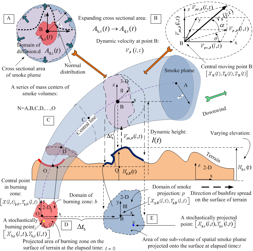 | Figure 1. normal distribution of temporal and spatial dispersion at cross section of smoke plume; (B) resolve velocity of geostrophic wind acting on center of mass of smoke plume; (C) smoke plume disperses downwind and correlates with bushfire spread on ground; (D) domain of burning zone; (E) domain of smoke plume projection |
The coordinates II is spherical coordinates. Selecting spherical coordinates is useful in estimating surface area of head of each smoke plume and its volume. Its shortcoming is that it is difficult to determine the spatial position of particles in the smoke plume because of no information about radius for each particle. To overcome it, the cylindrical coordinates thus coordinates IV (see Figure 2(B)) is chosen to trace the same observed particle shown by the coordinates II.
2.1.3. Spatial Projection Coordinates
The spatial projection coordinates thus the coordinates III (See Figure 1(E) and Figure 2(B)) is two-dimensional (2-D) coordinates. In practice, the spatial position of smoke plume in horizontal direction cannot be determined by itself. It is usually confirmed by 2-D projection coordinates on the ground. Once the horizontal position of a point in the spatial projection coordinates is confirmed, its elevation and the effective height of smoke plume over the surface of terrain can be therefore determined. Similar to spatial moving coordinates, the spatial projection coordinates III is expressed as [Xp(l,t),Yp(l,t)] (See Figure 1(E)), where the subscript p denotes the domain of projection p, on which smoke plume is projected. The parameter l is a variable representing a dynamic height of particles in smoke plume. It is to be discussed later.Both coordinates II and IV (See Figure 2 (A) and (B)) belongs to curvilinear coordinates because the particles in smoke plume are traced as flowing points in the fluid in this research. Hence, the smoke plume is treated as a fluid. The coordinates II and IV are built on the center of mass (N).
2.2. Specify Absolute and Relative Motion
One of most important issues in this research is specifying the type of motion for observed objects before modelling them. Several coordinates built in the last section are used for observing and depicting the motion of objects.The principle of classifying absolute and relative motion in terms of the position where the observer stands is also suitable for modelling the self temporal-spatial dispersion of particles in the smoke plume. For the particles in one sub-volume of smoke plume described by coordinates II, there are two types motion for them: absolute and relative motion. The motion of particles located in the coordinates II relative to the coordinates I is absolute, however the self-diffusion of those particles in smoke plume relative to coordinates I is relative.
2.3. On Spatial Location of Center of Mass
Strictly speaking, the spatial position of the center of mass for each sub-volume of smoke plume varies with respect to the elapsed time due to its self-diffusion and unmeasurable in reality. However, with smoke plume dispersion downwind, each center of mass is assumed as remaining in a central line: AO (see Figure 1(C)). Thus self-diffusion occurs around each center of mass (N). It may be easier to decide an azimuth for the assumed central line by means of measurement or using angle between burning and smouldering zone, of difficulty is to deal with the vertical position of each center of mass. In practice, there are two approaches in determining the spatial location of the center of mass (N). Under condition of that the direction of smoke plume dispersion has been confirmed, one manner is determining the center of mass (N) on the central line according to average velocity of smoke plumed dispersion first, and then the spatial position of particles in the sub-volume of smoke plume is determined by distributing them around the center of mass (N). Another is to distribute particles in the sub-volume of smoke plume first, and then the spatial location of center of mass (N) on the central line in vertical direction is assessed by the stochastic distribution of particles, it can be approximately located in the center of one sub-volume of smoke plume. The former is based on the observation from the coordinates I; the latter is based on the local observation from curvilinear coordinates thus the coordinates II and IV. The former is similar to Lagrangian method in investigating fluid dynamics; the latter is analogous to Eulerian method.The advantage of using the latter technique is that the local elevation of each particle in the sub-volume of smoke plume can be considered precisely. Accordingly, the latter manner is to be adopted in this research.
2.4. Define Domains
However, in reality, both smoke plume dispersion and bushfire spread are very complicated processes. Except for building several coordinates to describe the absolute and relative motion of particles in their temporal-spatial dispersion, another important approach is to define and classify the domains of observed objects in different regions so as to trace the horizontal motions respectively. Once the relevant horizontal domain is confirmed, the corresponding elevations of particles are also able to be considered. In Figure 1, there are two main types of domain. The domain of burning zone: b (see Figure 1(D)) is used to depict bushfire burning spots and their spread. The domain of smoke plume projection: p (see Figure 1(E)) is an area which is formed and projected by particles in each partitioned smoke plume. Both of two domains are formed stochastically. This is because the behaviour of bushfire spread in landscape and smoke dispersion in sky is a stochastic process respectively. However, in modelling, the relevant elevations located in the domain of projection p and burning zone b must be taken into account respectively when the heights of particles are involved in. Because the domain of p and b is only a horizontal and polygonal area, they do not provide any information in vertical direction.Other domain defined in this paper is domain of diffusion: d and domain of smoke head area: h and domain of unit surface: u respectively (see Figure 2 (A)). The domain of diffusion: d is used to illustrate the radial diffusion of smoke plume (see Figure 1(A)). Those domains are only used to precisely explain how smoke plume diffuses radially, how the front head of smoke plume disperses downwind and their relationship. As seen, the domain correlates with geometric feature of terrain and temporal-spatial position of particles.
2.5. Define Dynamic Height
In order to illustrate relationship between domain and height, a variable l(t) is introduced for observing the variation of height of smoke plume (see Figure 1 (C) and Figure 2(B)). It represents a dynamic height thus the variation of height of smoke plume rising from ground plus the corresponding elevation with respect to time t. When l(t) is equal to the elevation Hp,c(t), it means either bushfire spread on the surface of terrain or smoke plume just rise from ground. On the other hand, the variable l(t) is larger than elevation; it is also used to indicate the variation of magnitude of geostrophic wind with respect to the height. However, such a dynamic height is related to time t in the process of smoke plume rising from ground. Nevertheless, all cases discussed in this research are associated with the time t and the velocity of geostrophic wind. For the sake of simplicity, l(t) is written as l.
2.6. Detail Elapsed Time
In the modelling, the elapsed time t is one of important concepts and parameters, which is used in different aspects.The bushfire spread is a very complicated process. Although it can be classified into several sub-processes, all of them take place simultaneously. Therefore the elapsed time has different physical meaning in terms of specific case. The elapsed time can be renamed as the time of burning, bushfire spread, smoke plume dispersion and smoke plume self-diffusion respectively. Furthermore, any sub-processes can be also integrated and analysed by elapsed time and time interval if there exists potential correlations amongst them. The elapsed time t is usually assessed by the burning time interval Δtb (or Δt) counted from t =0 starting at the point O downwind in this research (see Figure 1(D)). However, the time interval Δt can be selected from any two elapsed time points to count how much time is consumed to finish a specific sub-process. The following cases explain how the elapsed time and time interval involves in modelling and interpreting a specific process.
2.6.1. Elapsed Time Applied in a Burning Zone
The elapsed time represents that the local burning and bushfire spread time relative to the coordinates I respectively. In this case, bushfire spread mainly depends on local distribution of vegetation in landscapes and local geographic location.Accordingly, assume that a stochastic distribution of burning spots happens in an existing burning zone or domain, then the burning and spread time is used to calculate and describe how long the part of vegetation in the currently burning zone is burnt and how fast or far the burning zone moves forwards downwind within the time interval respectively.
2.6.2. Elapsed Time Applied in a Smoke Plume Diffusion
In this case, the elapsed time describes how fast smoke plume dispersion and smoke plume self-diffusion take place from the original state respectively. Both of them are relative to the coordinates I.
2.6.3. Elapsed Time Applied in Multiple Processes
Because the bushfire spreading on the ground and plume spatial diffusion is a simultaneous process, in the same time interval Δt , the elapsed time can be used to calculate the horizontal (thus point: O→B) and vertical (thus point: Q→B) displacement of smoke plume(see Figure 1 (C)) and its self-diffusion (cross sectional area:  )(see Figure 1(A)), where the subscript d and c denotes diffusion of smoke plume and any points or positions of burning spot or diffusing particle in the current domain respectively.The expansion of cross sectional area for a smoke plume can be thought of as a process that the cross sectional area of smoke plume is enlarged from Ab,c (t) in burning zone at time t= 0 to Ad,c(t) at time t=t and a spatial position.
2.7. Combined Subscripts
The combined subscripts used for a specific parameter in this paper are to confine and describe a specific process or link it to others. For instance, the term Ab,c (t) means that the arbitrary and sectional area of smoke plume c in the currently burning zone b at time t and it expands to be Ad,c (t) at a new observed spatial location and one time t due to self-diffusion of smoke plume d. It is similar to other cases in the context.The more detailed illustration about subscripts is shown in Figure 1and Figure 2.
2.8. Conversion of Coordinates
Of importance in modelling temporal-spatial dispersion of smoke plume is to obtain its physical and physiochemical properties for further investigating how it impact on environment and vegetation in smouldering zone. It is not so difficult to estimate geometric properties in terms of designed model shown in Figure 1(A) and (C) or Figure 2 (A) and (B). The spherical model is especially suitable for describing the geometric shape of smoke plume. The cross sectional area and its surface area and volume of each head of smoke plume can be easily estimated by its radius  The radius shown by equation (1) is suitable for modelling general case of smoke plume.
  | (1) |
Where 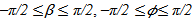 for hemisphere However, as seen from equation(1), the main problem is that it is impossible to determine both the temporal-spatial position for each spherical coordinates and the temporal-spatial position of particles of smoke plume stochastically distribute in each spherical coordinates.To overcome this difficulty, the best manner is conversion of coordinates. Hence, the observed objects in spherical coordinates are transferred into cylindrical coordinates. The observed objects in cylindrical coordinates can be investigated by combining it with its domain of projection p. In this approach, the temporal-spatial location of moving point (e.g. point B) [Xp,B(t), Yp,B(t), Zp,B(t)] is transferred into and considered and replaced by the corresponding point B [Xp,B(l,t), Yp,B(l,t), Zp,B(l,t)] in the cylindrical coordinates (see Figure 2 (A) and (B)). Such a process can be expressed by equation (2).
 | (2) |
Similar to dynamic and stochastically distributed particles, their transfer can be shown by equation (3). | (3) |
In the coordinates IV, the massive particles form a lot of cylinders. The trajectories of them can be traced and described by equation (4). | (4) |
 | Figure 2. coordinates conversion between spherical and cylindrical coordinates |
Where, the angle ω ranges  From equation(4), it can be easily discovered that the trajectories of particles in coordinates IV are related to their dynamic heights l, those also link to their varying elevations Hp,c(t) located within the domain of projection p.On the basis of such a transfer, the complicated case is dramatically simplified. It is able to 1). accurately establish relationship between the dynamic heights l of particles in smoke plume and their corresponding elevations Hp,c(t).2). effectively calculate their horizontal displacement within a time interval Δtb.More detailed discussion is to be implemented in part 2.
2.9. Concept of Geostrophic Wind
The geostrophic wind caused by the rotation of the earth and pressure gradient between two arbitrary isobars in the atmosphere. At ground level, the existing frictional force slants the geostrophic wind (see Figure 3(B)), so actual velocity Vact. ,geo (the subscript act and geo denotes actual and geostrophic wind respectively) is approximate to 40 percent of the one of the geostrophic wind. At high level, the friction is reduced[13], in other words the velocity of the geostrophic wind Vgeo is increased (see Figure 3(A)). The velocity of the geostrophic wind Vgeo can be estimated by equation (5). | (5) |
Where•ρ is the density of air.•  is the angular velocity of the earth; its magnitude is 2π∕24 rad h-1.•
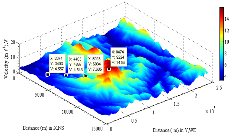
  is the latitude. • G is the pressure gradient, which equals the pressure force P acting on a unit cub of air, thus G=ΔP∕H, in which ΔP is the pressure difference between two arbitrary layers (isobars) with corresponding distance H (see Figure 3 (B)).For the practical purpose, the pressure P decreases 1.3123 Pa m-1 ascent near the surface of the earth[13].Such a fact is useful in calculating Vgeo by means of equation (5) and DEM.The result of the actual velocity of geostrophic wind Vgeo per 100 meter ascending shown in Figure 4 is assumed that
  = 1.166 kg m-3 at 30 °C,
  As seen, the Vgeo is increased with elevation at the ground.However, the density of air varies with increasing height; the actual Vgeo at high level differs from the one at ground level.
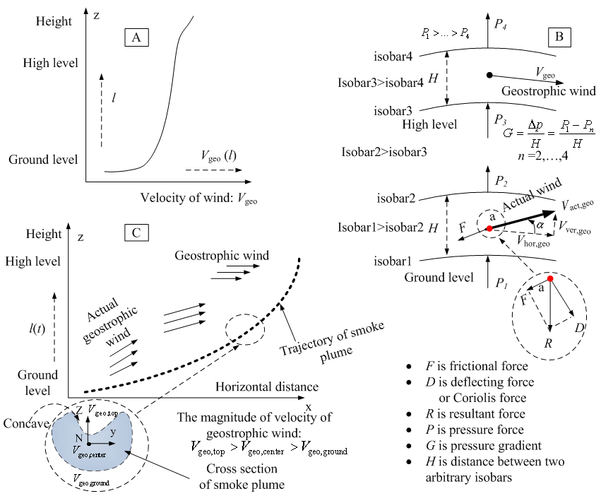 | Figure 3. (A) geostrophic wind varies with height; (B) trajectory of smoke plume influenced by geostrophic wind; (C) formation of geostrophic wind |
 | Figure 4. variation of geostrophic wind velocity with elevation per 100 meter |
2.10. Relate Geostrophic Wind with Dispersion of Smoke Plume
In reality, the geostrophic wind plays a prominent role in bushfire spread and dispersion of smoke plume. The velocity is a vector. Therefore at ground level, the velocity at a dynamic point B (see Figure 1and Figure 2(B)) VB(l,t) can be resolved into several components in multi-direction according to its azimuth(θ) and elevation angle (α) (see Figure 1(B)). The manner of estimating θ can be obtained by either measurement or designed angle downwind.As to the angle α, it is usually 25 to 35°[13]. However, it may be slightly different in the case of large scale bushfire spread.Each dynamic component of velocity of geostrophic wind thus Vpz,B(l,t) and Vpx,B(l,t), Vpy,B(l,t) is useful in estimating vertical and horizontal displacement of smoke plume based on its dynamic height l and its domain of projection p or burning zone b. Actually, velocities of any particles in smoke plume are able to be treated in the same manner.
2.11. Define Dynanic Diffusion Coefficents and Ratio of Geostrophic Wind
In modelling bushfire spread, many complicated cases are encountered especailly in estimating how fast bushfire spread on the ground and smoke plume disperse in different direction. It is impossible to measure them directly. In order to resolve encountered problems and simplify the complicated cases, the effective manner is introducing different dynamic diffusion coefficient and a specific ratio to detail different process. In this research, consider the diffusion velocity of smoke plume in vertical and horizontal direction, the velocity of self-diffusion and the ratio of real velocity of geostrophic wind to that of geostrophic wind with respect to height is different respectively, these cases should be dealt with separately. Because they are involved in a dynamic process, the following relvent equations relying on the elapsed time t and dynamic height l(t) in different cases are proposed.Case 1: horizonatal diffusion coefficent τ(t),which can be expresed by equation(6). | (6) |
Case 2: vertical diffusion coefficent λ(t), which can be shown by equation(7).  | (7) |
Case 3: self-diffusion coefficent  which can be shown by equation
 | (8) |
Case 4: the ratio of Vactual,geo to Vgeo : ε(l), which can be discribed by equation(9). | (9) |
The results from equation (6)−(9) are displayed in Figure 5(A)−(D).The spatial movement of smoke plume is affected by increasing magnitude of velocity of geostrophic wind Vgeo(l) with respect to height l (see Figure 3(A)). However, these cases require to be separately discussed as follows.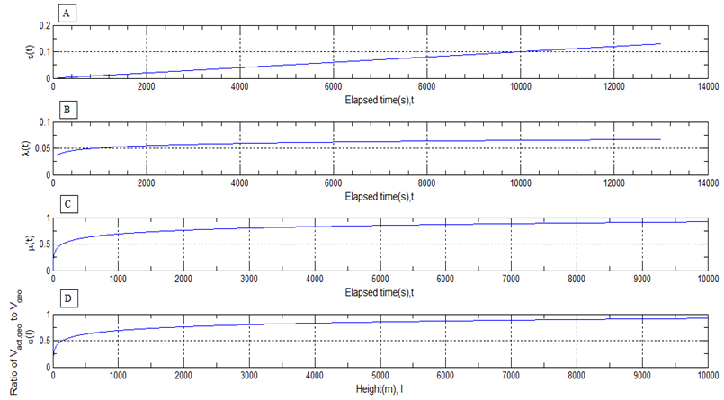 | Figure 5. (A) horizontal dynamic diffusion coefficient τ (t); (B) vertical dynamic diffusion coefficient λ (t); (C) dynamic self-diffusion coefficient μ (t); (D) dynamic ratio of geostrophic wind ε(l) |
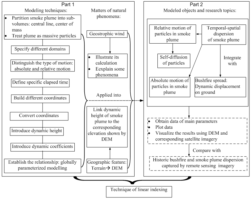 | Figure 6. summarize main process of modelling temporal and spatial dispersion of smoke plume and their correlation |
1). The reason why the horizonatal coefficent τ(t) is linear with the time t in the case 1 is that it only influences on the horizontal displacement of the center of mass of each sub-volume of smoke plume in the modelling. The maginitude of the horizontal displacement increases with respect to the increasing spatial volume of smoke plume due to the self-diffusion of particles. The fact is that the direction of geostrophic wind gradually alters to be parallel to the surface of the earth and its magnitude increases dramatically over 1000 meters because the frictional force is reduced[13]. Therefore the absolute velocity of smoke plume is increased with the change of geostrophic wind. It appears a linear relationship with the velocity of geostrophic wind.2). The situation in the case 2 is more complicated. The particles in smoke plume are in effect affected by at least four different forces such as Coriolis force, gravitational force, buoyancy force, thermal gradient force, centrifugal force, pressure gradient force in the process of smoke plume ascent. It is difficult to assess how those forces affect on the vertical velocity of smoke plume. Consequently, the vertical diffusion coefficient λ(t) is introduced, and it is assumed that it appears the relation of natural logarithm with time t. It can be used to assess how fast the smoke plume rises from the ground. The vertical diffusion coefficient λ(t) approaches to a constant with respect to increasing height l(t) and elapsed time t because of the effect of geostrophic wind.3). The self-diffusion coefficient  in the case 3 expresses how much the particles are resisted by ambient air in the process of temporal and spatial diffusion of smoke plume. As mentioned above, the self-diffusion coefficient
  is used for the relative motion of particles which is different from the absolute motion of particles shown in the case 1 and 2 respectively. Similarly, appear the relation of natural logarithm with time t. Only difference is that its magnitude is smaller than that in case 2 because the relative motion is always slower than the absolute motion. 4). The dimensionless ratio of Vact,geo to Vgeo thus ε(l) in the case 4 varies with the dynamic height of smoke plume l (t). Applying ε(l) to Vgeo is able to modify the actual velocity of geostrophic wind in time. The ε(l) is calculated by equation(9). The Vgeo is greatly influenced by the frictional force at ground level (below 1000 meters). As seen from Figure 5 (C), ε(l) approaches to a constant when the smoke plume ascends over 3000 meters, because the frictional force is negligible. Note that above introduced parameters are all dimensionless and adjustable. They are in fact able to be regarded as dynamic resistance coefficients if the velocity of geostrophic wind is treated as criteria of quantity. However, in a specific case, for example the self-diffusion coefficient can be thought as the coefficient of expanding the volume of smoke plume. The dynamic coefficients not only simplify complicated cases but also make the velocity of temporal-spatial dispersion of smoke plume be forecast-able.
2.12. Linear indexing applied in Modelling
The technique of linear indexing has been introduced and applied into tracing bushfire spread on ground by author[14, 15]. This powerful technique is also able to be applied into modelling the spatial dispersion of smoke plume. The reason is that the terrain of landscape is formed by matrix-based DEM and smoke plume disperses over that terrain. Therefore, the horizontal displacement of smoke plume is in fact traced by linear indices. On the other hand, they correlate them with corresponding elevation of DEM. The dynamic height of smoke plume over the surface of that terrain is therefore introduced to confirm the spatial position of particles located in smoke plume in three-dimensional direction.
3. Conclusions
The main feature of temporal and spatial dispersion of smoke plume is dynamic. The most difficult is accurately positioning it. Firstly, the idea of modelling it is that assume1. The smoke plume is regarded as consisting of a number of fine and same size particles.2. The smoke dispersion is performed downwind and present normal distribution in cross direction.Then, to confirm the spatial position of those particles over landscape, the elevation of DEM is considered. Because the vertical displacement of those particles is related to the geogstraphic wind, the magnitude of displacement for each particle in vertical direction is then connected to it. On the other hand, the particles are also influenced by many forces over surface of terrain; they could float up and down, then additional parameter dynamic height is then introduced. However, parameters in vertical direction need to be decided by the corresponding horizontal displacement. The horizontal component velocity for those particles can be gained by resolving the velocity of geostrophic wind as well. In order to determine horizontal position projected onto the terrain, the concept of domain is then introduced. This concept is widely expended to the other fields in the modelling. On the basis of the physical characters of smoke plume dispersion, more parameters are introduced one by one to consist with real situation. However, some parameters like different dynamic diffusion coefficients are made only for easily modelling according to fluid and meteorological features. No existing experimental data can be referenced. Finally, two important tricks applied in this modelling should be further pointed out.1. Obtaining physical properties of smoke plume such as expanding surface area and volume and correlating vertical height of particles with elevation of terrain have to rely on the conversion of coordinates.2. Linear indexing is thoroughly applied into tracing motion of smoke particles, transferring data and mutually displaying results between DEM and satellite imagery. Hence, all performance in modelling is carried out in the same matrix, mathematically speaking.Above two key points are hidden in each step of modelling.The main correlation between them is briefly summarized in Figure 6. The detailed procedure of modelling is to be implemented in the part 2.
ACKNOWLEDGENTS
Author wants to offer special thanks to Professor Jing. X. Zhao at Shanghai Jiao Tong University for supplying desired data used in this research.
References
| [1] | J. B. Kirkpatrick, J. B. Marsden-Smedley, and S. W. J. Leonard, "Influence of grazing and vegetation type on post-fire flammability," Journal of Applied Ecology, vol. 48, pp. 642-649, 2011. |
| [2] | R. K. Smith, "Radiation effects on large fire plumes," Symposium (International) on Combustion, vol. 11, pp. 507-515, 1967. |
| [3] | L. Orloff, A. T. Modak, and G. H. Markstein, "Radiation from smoke layers," Symposium (International) on Combustion, vol. 17, pp. 1029-1038, 1979. |
| [4] | L. F. Radke, A. S. Hegg, P. V. Hobbs, and J. E. Penner, "Effects of aging on the smoke from a large forest fire," Atmospheric Research, vol. 38, pp. 315-332, 1995. |
| [5] | G. E. Willis and J. W. Deardorff, "On plume rise within a convective boundary layer," Atmospheric Environment (1967), vol. 17, pp. 2435-2447, 1983. |
| [6] | B. R. Morton, "Modeling fire plumes," Symposium (International) on Combustion, vol. 10, pp. 973-982, 1965. |
| [7] | M. J. Pilat and D. S. Ensor, "Plume opacity and particulate mass concentration," Atmospheric Environment (1967), vol. 4, pp. 163-173, 1970. |
| [8] | D. Weihs and R. D. Small, "An approximate model of atmospheric plumes produced by large area fires," Atmospheric Environment. Part A. General Topics, vol. 27, pp. 73-82, 1993. |
| [9] | G. N. Mercer and R. O. Weber, "Fire Plumes," in Forest Fires, A. J. Edward and M. Kiyoko, Eds. San Diego: Academic Press, 2001, pp. 225-255. |
| [10] | R. G. Rehm, "The effects of winds from burning structures on ground-fire propagation at the wildland-urban interface," Combustion Theory & Modelling, vol. 12, pp. 477-496, 2008. |
| [11] | Y. S. Chung and H. V. Le, "Detection of forest-fire smoke plumes by satellite imagery," Atmospheric Environment (1967), vol. 18, pp. 2143-2151, 1984. |
| [12] | A. Lavrov, A. B. Utkin, R. Vilar, and A. Fernandes, "Evaluation of smoke dispersion from forest fire plumes using lidar experiments and modelling," International Journal of Thermal Sciences, vol. 45, pp. 848-859, 2006. |
| [13] | S. Petterssen, Introduction to meteorology, 1st ed.: The McGraw-Hill Book Company,Inc, 1941. |
| [14] | C. Y. H. Jiang, "Modeling Bushfire Spread Based on Digital Elevation Model and Satellite Imagery: Estimate Burning Velocity and Area," American Journal of Geographic Information System, vol. 1, pp. 39-48, 2012. |
| [15] | C. Y. H. Jiang, "Digital Elevation Model and Satellite Imagery Based Bushfire Simulation " American Journal of Geographic Information System, vol. 2, pp. 47-65 2013. |
 Abstract
 Reference
 Full-Text PDF
 Full-text HTML