Carl Y. H. Jiang
Centre for Intelligent Systems Research, Deakin University, Victoria, 3216, Australia
Correspondence to: Carl Y. H. Jiang, Centre for Intelligent Systems Research, Deakin University, Victoria, 3216, Australia.
| Email: |  |
Copyright © 2012 Scientific & Academic Publishing. All Rights Reserved.
Abstract
The effect of terrain on mass and heat transport of smoke plume has been neglected for a long time. A novel manner of investigating it has been proposed by integrating terrain with spatial position of smoke plume by means of Gaussian distribution. Based on unique features of digital elevation model and satellite imagery, several necessary parameters to calculate distribution of mass and heat being carried by smoke plume were capable of being obtained. The results of modelling have effectively indicated some phenomena which have not been discovered and reported. The new approach of being expressed by geomorphologic parameters is useful to not only understand how mass and heat transport of smoke plume are affected by terrain but also estimate how mass and heat impact upon the vegetation closed to burning spots. The relation between smoke plume and burning zone in mass and heat diffusion has been closely correlated.
Keywords:
Smoke Plume Modelling, Digital Elevation Model, Mass and Heat Transport, Bushfire, Remote Sensing Imagery
Cite this paper: Carl Y. H. Jiang, Effect of Terrain on Mass and Heat Transport of Smoke Plume Based on Geometric Properties of Digital Elevation Model and Satellite Imagery, American Journal of Geographic Information System, Vol. 2 No. 4, 2013, pp. 67-81. doi: 10.5923/j.ajgis.20130204.01.
1. Introduction
Bushfire is a process of combustion in which transport phenomena have widely involved. Smoke plume is a by-product produced by combustion, which implies many phenomena and uncertain factors. Therefore, relevant researches have different focuses. Studying combustion has been implemented by many researches for many years[1-3]. However bushfire has unique features which are different from industrial combustion. Bushfire happens in an open natural environment. Therefore several researchers have developed the bushfire models based on theories of transport phenomena and thermodynamics[1-4]. In these researches, researchers have also paid a lot of attention to the studies of smoke plume[5-7]. However, investigating smoke plume has been remained within theoretical modelling based on laboratory scale experiments although the effect of terrain on bushfire and smoke plume has already been realized by all researchers in this field. So far, the studies have not been reported on the basis of real terrain.
2. Methodology
2.1. Features of Research
In this research, the concentration is to be drawn to investigating some unknown fact happening in smoke plume dispersion accompanying with bushfire spread in landscape, hence how terrain affects on mass and heat distribution of smoke plume when it rises from ground. This topic has been ignored by assuming terrain is flat in the historical relevant researches. Because modelling is based on digital elevation model (DEM) and corresponding satellite imagery, the manner to be proposed in this research is novel and unique. The elevation supplied by DEM becomes valuable when applying Gaussian distribution into model smoke plume. On the other hand, one important parameter such as surface area is also able to be obtained by combining DEM and its remote sensing imagery; it becomes possible to effectively calculate mass and heat transport being carried by smoke mixture. Inversely, the distribution of them is helpful to provide useful information in estimating pollutant and heat how to impact environmental vegetation.
2.2. Objectives and Scope of Research
The objectives of this research are represented as follows.1. Review geomorphologic parameters and how they are extracted from DEM; it includes mass and heat transport existing in general combustion. Classify mass and heat for bushfire and smoke mixture in terms of concept of source and sink so as to easily model.2. Review Gaussian distribution in the statistics for developing new model on the basis of new ideas.3. Discover how the standard deviation of Gaussian distribution and mass, heat diffusivity is correlated mathematically and how to locate expected values into DEM based modelling.4. Find out how burning zone and smoke plume are connected in form of mass and heat transport.5. Estimate how terrain affects the distribution of mass and heat when smoke rises from ground. There are two approaches to be implemented. One is using traditional model to calculate for comparison; another is to apply proposed model into this performance. The explanation for modelling is based on the existing satellite imagery of bushfire.
2.3. Geographical Location for Modelling
Estimating mass and heat released from bushfire in this modelling is based on the place where bushfire often took place historically in Victoria, Australia. The geographical location (-36°70'10" S, 146°44'30" E; -36°83'60" S, 146°71'00" E) is shown by Figure 1. The distribution of vegetation is stored in the satellite imagery captured by the satellite LANDSAT and the feature of terrain is illustrated by the corresponding DEM (SRTM3 offered by USGS) in Figure 2. In Figure 1, the bushfire spread in landscape downwind and smoke plume spatial dispersion were modelled previously. In this research, the concerned topic is to focus on one of burning zones and smoke plumes as respectively indicated by circles shown in Figure 1 to investigate how the distribution of mass and heat being carried by smoke plume is performed spatially and potential correlation between it and burning zone. The results of modelling are displayed and calculated by MATLAB®.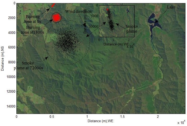 | Figure 1. selected satellite imagery for modeling smoke plume |
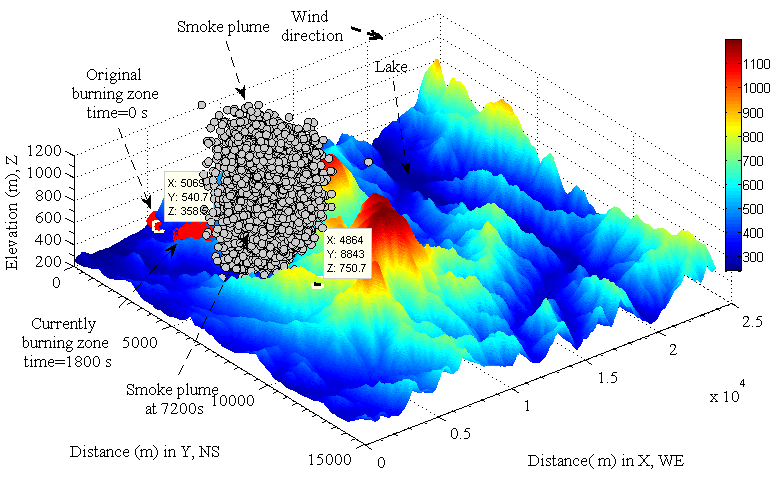 | Figure 2. corresponding DEM for modeling smoke plume |
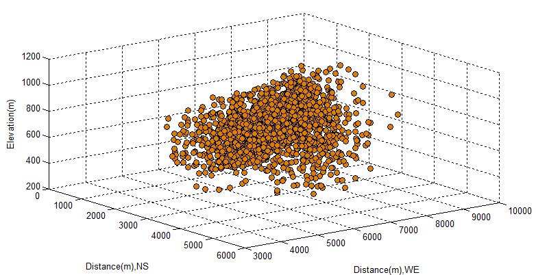 | Figure 3. detailed elevation of bushfire spots in modeling |
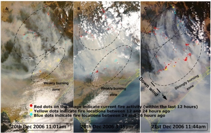 | Figure 4. December 2006 Victorian bushfire satellite images, Australia[5] |
Because fully modelling three-dimensional (3-D) case, it requires massive physical computer memories, modelling is only confined to two dimensional cases. However, this approach does not affect final results. Furthermore, additional energy source such as solar radiation is not to be considered in this research.To trace overall smoke plume correlates with elevation of terrain, it results in massive data to be involved in. In this research, only partial smoke plume over burning zone is considered. The detailed elevation of it is presented in Figure 3. As seen, the distribution of vegetation at the selected burning zone is uneven.
2.4. Smoke Plume Captured by Satellite Imagery
The modelling smoke plume is based on historical bushfire happened at the east coast in Australia. The two-dimensional satellite imageries are shown in Figure 4. An intuitive understanding how smoke plumes were generated by bushfire (red) are provided. It is useful to guide how model bushfire spreads, smoke dispersion especially in assessing how terrain affects distribution of mass and heat transport of smoke plume spatially, and reversely understanding how it impacts upon the vegetation distributing on terrain.
3. Fundamentals of Digital Elevation Model and Satellite Imagery
3.1. Mathematical Expression of Terrain
The surface of terrain is able to be described by continuous mathematical functions. In the following case(see Figure 5), if a boundary function b for boundary function C in domain D is given, thus y=b(x), then the area of D is given by equation (1) in terms of Green theorem and the geometric properties of trapezoid[6].  | (1) |
The area of surface over D is  | (2) |
Where, the f x2 and f y2 is the second order derivative of a continuous surface function f(x,y) in x and y direction respectively. Very obvious, the elevation z in a given domain can be expressed as  | (3) |
The elevation z represents a series of points consisting of a smooth and continues surface of terrain.If function f(x,y) is equal to an arbitrary constant, then at the point P (see Figure 5), along its normal, it will yield its gradient shown as  | (4) |
Where, the i, j is the unit vector and the f x ,f y is the first order derivative of a surface function in x and y direction respectively.The norm of equation (4) is named as slope, thus equation(5).  | (5) |
The slope represents the variety of elevation per unit length. Its corresponding angle is shown in the equation(6). | (6) |
The range of slope angle is from −90° to 90°.When f x≠0, then the aspect  (see Figure 5) is expressed as
  | (7) |
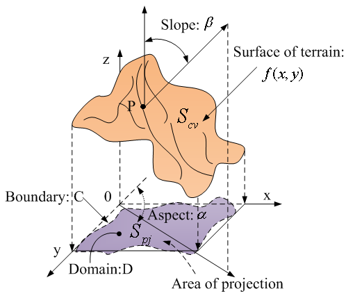 | Figure 5. Schematic illustration of geomorphologic parameter |
The aspect is the azimuth of the slope direction and its angle ranges from 0° to  . In other manner, the aspect is also thought of as the direction of the biggest slope vector on the tangent plane projected onto the horizontal plane.Another useful concept is roughness. The unit roughness Rk is defined as the ratio of the surface area Scv to its projection onto the horizontal plane Spj for the kth unit of surface area (see Figure 1). The area of surface is portioned into k regular size sub-elements.
 | (8) |
The concept of slope, aspect and roughness is an important respectively.However, the analytical solutions to them are difficult to be obtained in practice; usually they can be resolved and applied in the form of numerical form.
3.2. Extract from Geometric Parameters from DEM
DEM is a common used data. Several valuable parameters mentioned above can be numerically expressed.Because the research is to focus on how terrain affects the distribution of mass and heat being carried by smoke plume, a window-like numeric manner of dealing with DEM is to be used. The maximum drop slope was proposed by researchers[6]. The local moving “window” is similar to the principal of filter used in digital image processing because both of DEM and digital imagery is based on a specific matrix. The DEM data “flows” into this window, the geomorphologic features of DEM such as slope and aspect are extracted.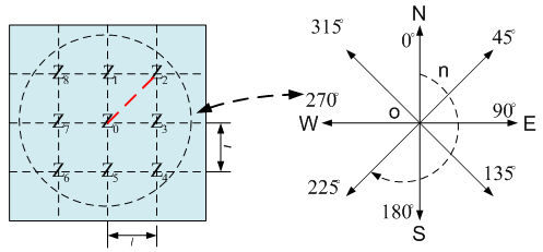 | Figure 6. a moving window of maximum drop slope |
The manner of maximum drop slope is selecting one cell as a centre of cell, its elevation Z0 is then compared with elevation Zn of neighbor cells clockwise (see Figure 6), n=1,2,…8.As mentioned above, the aspect is thought of as the direction of the biggest slope vector on the tangent plane projected onto the horizontal plane. Then, slope and aspect angle in manner of maximum drop slope can be mathematically expressed as follows. | (9) |
 | (10) |
 | (11) |
Where, l is cell size.When n is even number,  , otherwise j=1.The detailed explanation integrating above geomorphologic parameters with some features of satellite and application in modelling bushfire have been discussed by author[7, 8].
4. Basic Theories of Mass and Heat Transport
The mass transfer is visible in the form of smoke plume. However the heat transfer is complicated and invisible for human, it can be appeared in the form of both free convection and radiation. The energy not only can be carried by air (heat conduction) but also transported by gray gases (such as CO2) and fine granules in the smoke mixture. In other words, the energy can be stored and carried by the smoke mixture and distributed in air like the behaviour of smoke plume’s diffusion. According to Newton’s cooling law, the free convection of heat only affects the vegetation close to the burning zone rather than the one in remote zone. In order to investigate how the energy affects the remote vegetation, assume that the form of motion for spatial energy transfer is the same as smoke plumes’. In fact, mass and energy coexists. Such technical treatment is to be much easier to understand how the mass and energy density is decayed with the elapsed time respectively and how they impact upon the vegetation in remote zone. Both mass and energy density are extensive property rather than intensive property, thus they are varied with expanding volume and elapsed time.
4.1. General Conservation Equation of Mass and Heat
According to the concept of source and sink when mass and energy are transported (flow in or out) within two different systems, it can be described as the following equation. | (12) |
In which in general θ, η, t and z represent one conserved term (mass or heat), flux (of mass or heat), time and displacement in a one-dimensional system in the left hand of equation(12) respectively; in the right hand of it, Φ represents the source of mass or heat. The unit for the equation(12) can be like kg∙m-3∙s-1 for mass transport and kJ∙ m-3∙s-1 for heat transport respectively. In order to clearly illustrate physical meaning of variables, the S.I. units are supplied for them in the context; they are adjustable according to specific case in practice.Equation(12) is very useful to explain how mass and heat transport happening in bushfire and other equations’ derivation also relies on it. If the source term is equal to zero, then equation(12) become  | (13) |
Equation(13) is then named as a continuity equation. Hence, nothing (mass and heat) is created or destroyed. It is also useful in explaining and estimating the distribution of mass and heat when smoke plume disperses spatially.A. General Expression for Substance TransportIn general, for both mass and heat transport, in a one-dimensional system, they can be written as the following general equation[9-11]:  | (14) |
The coefficient A, B and C represents different physicochemical properties containing behaviours cause them respectively. B. Mass TransportIn the matter of the burning, which can be regarded as a process of chemical reaction, the bushfire produces a number of species; in general, it is not precise enough to define mass transport using concentration if the species in smoke is more than one. Instead, the mass fraction or molar mass fraction Ψi (i=1,2,…,g) is used to define mass transport. Then the expression of equation(14) combining with equation(12) becomes equation(15) between two systems and in one-dimensional direction. | (15) |
Where  is the mass diffusion coefficient or mass diffusivity for species i into the mixture of the other species in a given system, its unit is m2∙s-1. The superscript M indicates mixture in the context. ρ is total mass density, its u. nit is kg∙m-3.The term
  is the rate of production of species i in chemical reactions, its unit is kg∙m-3∙s-1.Where the mass velocity
  of the species i is composed of the mean mass velocity
  of the centre of mass of the mixture and a diffusion velocity
  (relative to the centre of mass) caused by molecular transport because of the concentration gradients of the species
  . The unit of both of velocities are m∙s-1. The relation between two types of velocity is expressed as
 | (16) |
In fact, there are two coordinates in above describing mass transport. Depending on how to observe the motion of substance, if the bushfire spot is selected as a stationary coordinates, the velocity of motion of one center of mass-based smoke plume is v. If the second coordinates is located at the center of mass, the diffusion velocity of species i is Vi.Therefore, equation(15) tells that the species i flows into one system into another. In the case of burning vegetation, it can be considered as that smoke (gaseous mixture) in the form of heat and mass fluxes from ground into sky, and then form smoke plume spatially and carry heat simultaneously. The unit for equation(15) can be kg∙m-3∙s-1, in the terms of that, it is easy to verify each term.C. Heat TransportIf the term Y in equation(14) denotes temperature T, then the heat transport between two systems is represented as(17).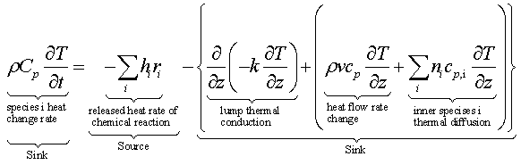 | (17) |
Where  is the specific heat capacity species i at the constant pressure. The unit of Cp is kJ∙kg-1∙K-1. The k is the heat conductivity of the species i mixture, its unit is kW∙m-1∙K-1.
  is the enthalpy of species i mixture, its unit is kJ. ni” is mass flux in the center of mass system is defined as.
 The mass flux ni” is kg∙ m-2∙s-1.Therefore, the unit for equation (17) is kJ∙m-3∙s-1.
4.2. Mass Diffusion and Heat Conduction Associated with Smoke Plume
In this research, studying the smoke plume produced by burning vegetation is the main topic. Although it is to be discussed separately, the smoke plume still has a close relation with the bushfire at the ground. Assume that1. Smoke plume is a continuous gaseous mixture fluid, which can be parted into a series of sub-volume with a center of mass (see Figure 7). 2. For a given sub-volume smoke plume, no chemical reaction takes place in inert mixture and density  of smoke mixture does not change with spatial distance.Based on those assumptions, from equation (15) and(17), it leads to generating following equations respectively:
 | (18) |
 | (19) |
Obviously, the equation (18) is Fick’s second law and the equation(19) is Fourier’s second law in one-dimensional form respectively. On the other hand, it can be seen that mass diffusivity of mixture DiM is equivalent to the thermal diffusivity α in form as follows.  Where k is thermal conductivity, W∙m-1∙K-1The unit for both DMi and α is m2∙s-1.Under such assumptions, although each sub-volume smoke plume is able to be independently carry out its mass transport and thermal conduction spatially, it naturally correlate with mass and heat flux produced by burning spot at ground with respect to time. The flow rate of them can be implicitly described by the following equations(20)−(21) respectively.
 | (20) |
Where the concentration of species i is 
 | (21) |
In equation(20) mi’ is mass transfer rate (kg∙s-1) of species i, which emits from a burning zone with the surface area Sb and rising with local geostrophic velocity vb; then the species i disperses from a given one smoke plume with volume Wsp. The subscript b and sp denotes burning and smoke plume respectively. In equation(21), q’ is heat flow rate (kJ∙s-1) accompanying with the mass fluid rises from ground with the difference of temperature ∆Tb.As seen from equation(20) and equation(21), once the smoke plume leaves from ground, no additional mass and heat from ground is added into each smoke plume. It independently carries out mass and heat transport spatially.On the other hand, one issue should be illustrated before further discussing smoke plume. At ground, in terms of equation (18) and(19), in semi-infinite media the concentration Ci distribution of species i in gaseous mixture(smoke) when its initial fraction Ci1 at initial time jumps to be Ci2, Ci2 > Ci1 due to instant mass diffusion can be expressed as follows. | (22) |
Similarly, the temperature T distribution of gaseous mixture can be shown as follows if the initial temperature T1 increases to be T2.  | (23) |
Both ς and ζ is a dimensionless variable having the following mathematical properties as | (24) |
 | (25) |
 | (26) |
The erf is an error function and erfc is a complementary error function.Also, erf(∞)=0 when ζ→∞, thus erfc(ζ)=1 according to equation(24). The mass and heat flux m”i and q” can be written as follows based on equation(20)−(23). | (27) |
Similarly | (28) |
The mathematical properties of equation (25)−(28) are useful to be further used in the following suction.D. Mathematically Correlate Mass Diffusion and Heat Conduction Second Law with Gaussian DistributionThe previous researchers[12-14] used to investigate the mass diffusion of smoke plume by means of Gaussian (normal) distribution appeared in statistics. The spatial mass diffusion and heat conduction of smoke plume is somewhat different from the cases of them happening at ground because they do not have a clear boundary and initial conditions spatially. Therefore to model concentration and heat distribution of smoke plume, it requires to build a central line based on the center of mass of each smoke plume. Then distribution happens radically along this line.The approach in statistics is that, in one dimension, for the a standard normal random variable with density function f(x), its expected value μ can be expressed as | (29) |
With | (30) |
Its variance σ2 is shown as  | (31) |
Because the density function f(x) is symmetric with respect to the y-axis in the x-y coordinates, then  When μ =0, then
 | (32) |
If let  then
then | (33) |
As seen, when x→+∞, u→+∞, σ2=1.Therefore, in general the normal density function with parameter μ and σ can be defined as follows in one-dimensional form. | (34) |
Equation(34) is also able to be extended. The two or three-dimensional form is shown as follows. | (35) |
 | (36) |
Now comparing equation (34)−(36) with equation (27)−(28) produces the following discoveries.In mass diffusion: | (37) |
In thermal diffusion: | (38) |
The unit for both σ and μ shown in equation(36)− (38)is m. Therefore the term of exponent in equation(36) is dimensionless and then the unit for equation(36) becomes m-3. On the basis of the unique feature of equation(36), its application in investigating smoke plume is to be further modified in the following section.
4.3. Concentration Distribution
A. 3-D Constant Source from Burning ZoneThere several Gaussian distribution-based models to describe the smoke plume. The smoke plume generated from ground is usually treated as a fluid in steady state, then the change of concentration with time is zero, furthermore, the diffusion of smoke plume in - x direction can be neglected because of the downwind (See Figure 7). Then the distribution of concentration of smoke plume is often expressed by equation(39)[15].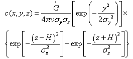 | (39) |
 | Figure 7. schematic illustration of smoke plume dispersing over terrain |
In which (See Figure 7), for smoke with constant source, the smoke plume is always described by using the effective stack height of smoke H, its unit is m. The v is the average wind velocity at stack height. G. is emission rate of source; its unit is kg∙s-1.σx, σy are the standard deviations of the concentration distributions in the crosswind and vertical directions respectively. The unit is m for them. x is the distance downwind from the stack; y is the crosswind distance from the plume center line and z is the vertical distance from ground level. The unit for them is m.B. Smoke Plume Based DistributionEquation (39) is established by assuming the ground is flat.In fact, the smoke plume especially caused by bushfire is seriously affected complex terrain. In order to set up the correlation of plume with elevation of terrain making use of the advantage of DEM, assume that1. The smoke plume is puffed from one burning zone within each time interval. 2. The mass and energy released from burning are remained in each smoke plume having different initial spatial surface area and volume and diffuse at specific spatial location.3. Smoke plume is composed of massive fine particles.4. The solar radiation is not considered.5. Each smoke plume has its own mass center forming a central line.Based on above basic assumptions and the concept of equation(36), the following results can be generated.1. The point (μx,, μy,, μz) represents a spatial point locating at a central line and specific time respectively.2. The vertical distance of each particle in each smoke plume z is equal to its vertical spatial position minus its corresponding elevation of terrain. If the diffusion in x-direction is not considered, the modification of equation(35) for spatial concentration distribution in y and z direction can be rewritten as follows. | (40) |
In which, M is total mass of each smoke plume, kg. σy, σz have the same meaning as ones defined above. A0 and Wsp are surface area of smoke plume at initial time 0, m2 and its spatially expanded volume at one specific time, m3 respectively, those two parameters can be yielded by other modelling. The unit of C(x,y,z) is kg∙m-3.The total mass M of each smoke plume can be obtained from equation(20) for species i within one time interval of burning ∆tb, s to produce it, which is shown by the following equation. | (41) |
In practice, directly setting up three-dimensional relation between smoke plume and landscape requires massive physical computer memory. Therefore the complex case is described by two-dimension based equation(40) without directly considering x-direction distribution of mass and heat.
4.4. Heat Density Distribution
Similarly, the heat density distribution and total heat being carried by each smoke plume and combining with equation(21) are shown as follows respectively. | (42) |
And | (43) |
The unit of E(x,y,z) and Q are kJ∙m-3 and kJ respectively.Up to this point, the necessary concepts for this research are already introduced. The results of modelling are to be displayed and discussed in the following section.
4.5. Estimate Diffusion Coefficients
In general, there exist two manners to estimate mass and thermal diffusion coefficients of smoke plume σx, σy, σz. One is using equation(37)−(38). Another is to use existing data and figures[16] (see Figure 8 and Figure 9). The latter manner is often applied in investigating mass diffusion in vertical and lateral direction.However, more precise manner is to use power law. | (44) |
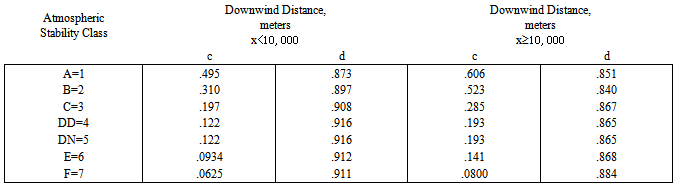
The values for a,b,c and d shown in equation(44) can be found in Table 1 and Table 2 according to downwind distance(see Figure 7).
5. Results and Discussion
5.1. Common Used Parameters and Values in Modelling
In the modelling, there are several parameters used in calculation. They are listed in Table 3. In which, v and vb are assessed by local geostrophic wind according to elevation and height of smoke plume when bushfire takes place at specific geographic location having burning area Ab. The manner of estimating above parameters has been introduced in the previous reports[7, 8]. αy, αz, Dy and Dz are mainly estimated by the thermal and mass properties of carbon dioxide (CO2)[17] at initial time. Similarly, ρ and Cp are modified by considering smoke plume as a gaseous mixture. Tb is a temperature jumping from ambient temperature to maximum burning temperature within a time interval when smoke rising from ground. A0 may be difficult to be assessed, which is approximately treated as 1 square meter in order for smoke to be physically observed at initial stage. 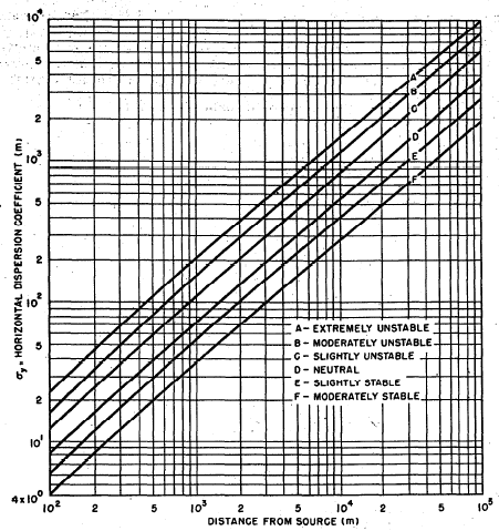 | Figure 8. vertical diffusion σz vs. downwind distance from source |
 | Figure 9. lateral diffusion σy vs. downwind distance from source |
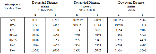
Table 1. power law exponents and coefficients for σy
 |
| |
|
Table 2. power law exponents and coefficients for σz
 |
| |
|
| Table 3. common mass, thermal and physical properties used in calculation |
| | Term | Symbol | Value | | Velocity of central line in x direction | v | 6.216 m ∙s-1 | | Smoke rising velocity in burning zone | vb | 3.101 m s-1 | | Effective stack height | H | 397.704 m | | Burning temperature | Tb | 1200 K | | Specific heat of smoke mixture at constant pressure | Cp | 1.047 KJ∙kg-1∙K-1 | | Density of smoke mixture in burning zone | ρ | 1.8864 kg∙m-3 | | Currently burning area | Sb | 2.8419e+06 m2 | | Thermal diffusivity in y direction | αy | 2.00e+06 m2 ∙s-1 | | Thermal diffusivity in z direction | αz | 3.190e+06 m2 ∙s-1 | | Mass diffusivity in x direction | Dy | 4.721e+06 m2 ∙s-1 | | Mass diffusivity in y direction | Dz | 2.560e+06 m2 ∙s-1 | | Initial surface area of smoke plume | A0 | 1.00 m2 |
|
|
The mass and heat emission rate produced by one given burning area Sb are presented in Table 4. Those data are calculated by using equation(20)−(21) and the corresponding data supplied in Table 3, and then applied into all calculations of mass and heat transport.| Table 4. calculated mass and heat emission rate for given burning area |
| | Term | Symbol | Value | | Mass emission rate | m. | 1.6256e+07Kg∙ s-1 | | Heat emission rate | q. | 4.8504e+10 KJ∙ s-1 |
|
|
5.2. Spatial Distribution of Concentration
Investigating how terrain affects distribution of concentration is carried out two approaches. One is using traditional equation(39) and supplied data in Table 3 and Table 4 for relevant parameters. The result is represented in Figure 10. σy and σz are assessed by using equation(37) and the relevant data are shown in Table 3.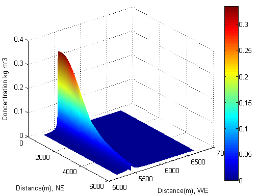 | Figure 10. concentration of smoke plume distributes without considering effect of terrain |
Another is using proposed equation(40) and relevant data supplied in Table 5. σz and σy are estimated by using equation (44) combining data supplied in Table 1and Table 2. In this case, the smoke plume is assumed as a moderately stable gaseous mixture, thus F type (see Figure 9).Table 5. parameters and values used for mass and heat transport calculation of smoke plume in two different cases
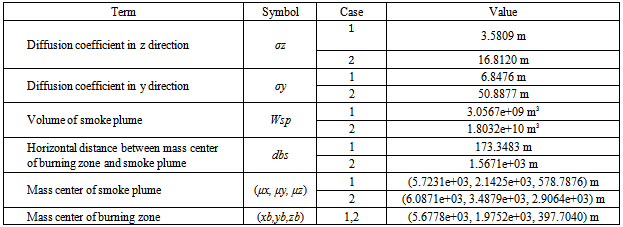 |
| |
|
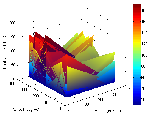
DiscussionThe results shown in Figure 11−Figure 16 provide the following information that 1. The distribution of mass is seriously affected by terrain described by geomorphologic parameters. 2. As seen from Figure 11 and Figure 14, the maximum concentration is presented in the location where it has maximum slope angle when smoke plume rising from ground.3. According to the principle of the maximum drop slope, the location having maximum slope accompanies with the maximum elevation. Therefore, the concentration of mass is always higher than one distributed in other place. Such phenomena have been approved by Figure 3, Figure 13 and Figure 16. 4. However, the aspects shown in Figure 12 and Figure 15) offer another important information, thus the maximum drop slope unevenly distributes in terrain. 5. For visible mass distribution, the complex terrain easily causes the turbulent state of smoke plume. In other words, the concentration distribution is uneven.Above fact can be approved by satellite imagery shown in Figure 4. As seen from it, the concentration distribution is seriously affected by adjacent hills (slopes) and varies with height.Traditional research manner is treating the distribution of smoke as being in idea state (see Figure 10 ). Therefore, the result shows very smooth and steady state. It results in a big error in estimating mass distribution in investigating smoke plume.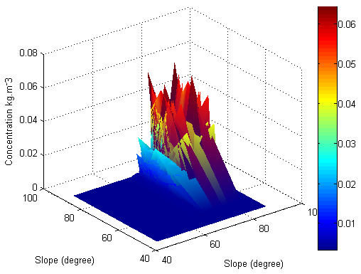 | Figure 11. concentration distribution affected by slope for case 1 |
 | Figure 12. concentration distribution affected by aspect for case 1 |
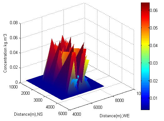 | Figure 13. concentration distribution affected by elevation for case 1 |
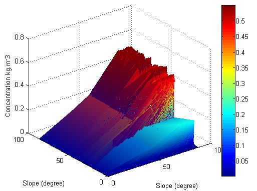 | Figure 14. concentration distribution affected by slope for case 2 |
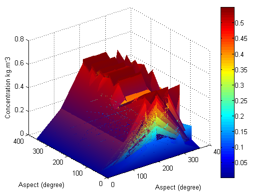 | Figure 15. concentration distribution affected by aspect for case 2 |
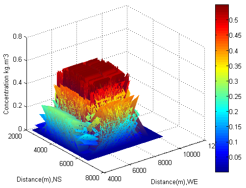 | Figure 16. concentration distribution affected by elevation for case 2 |
5.3. Spatial Distribution of Heat
As mentioned before, the heat transport is analogous to mass transport. The result shown in Figure 17 in a traditional manner is obtained by the one similar to equation(39). Nevertheless, the emission rate of source is replaced by heat q. supplied in Table 4. σy and σz are assessed by using equation(38) and relevant data shown in Table 3. The heat distribution is calculated by equation (42) using data supplied in Table 5 and assuming the heat loss and additional heat (such as solar radiation) are not considered.Discussion In according to the various results shown in Figure 18−Figure 23 and the feature of terrain described by Figure 3, it can be found that Heat distribution is also affected by adjacent hills (slopes)In terms of the scenario shown in Figure 4, heat conduction is also in a turbulent state; however it cannot directly be demonstrated by the current satellite imagery (Figure 4).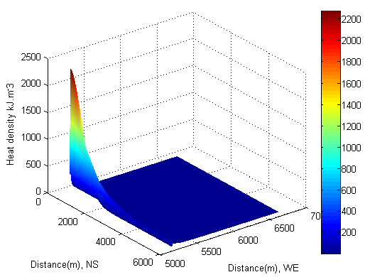 | Figure 17. heat of smoke plume distributes without considering effect of terrain |
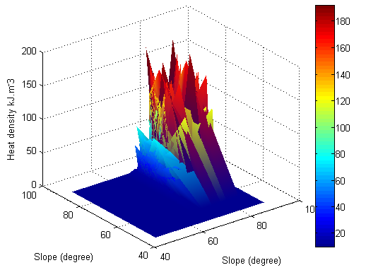 | Figure 18. heat distribution affected by slope for case 1 |
 | Figure 19. heat distribution affected by aspect for case 1 |
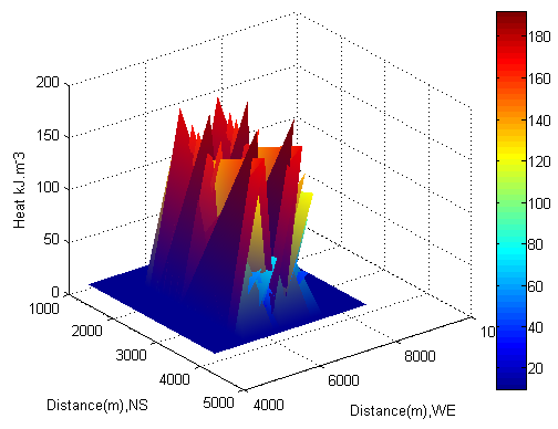 | Figure 20. heat distribution affected by elevation for case 1 |
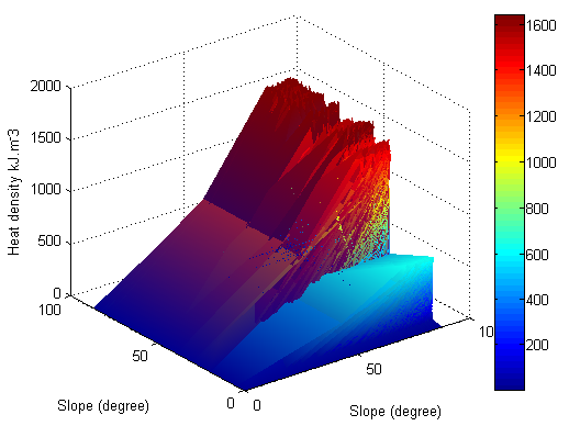 | Figure 21. heat distribution affected by slope for case 2 |
 | Figure 22. heat distribution affected by aspect for case 2 |
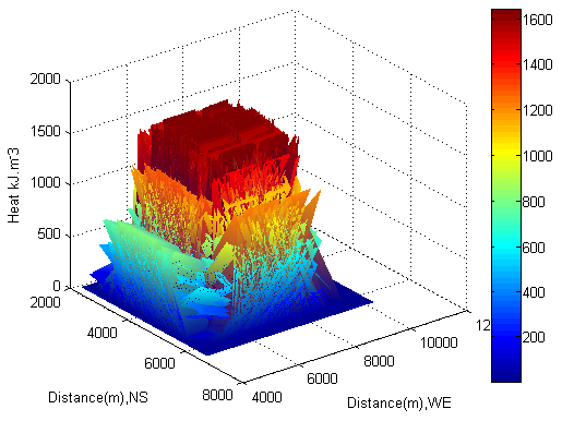 | Figure 23. heat distribution affected by elevation for case 2 |
6. Conclusions
A. Achievements in the ResearchThe effect of large scale terrain on the distribution of mass and heat being carried by smoke mixture has not been investigated for several decades although some researchers have already pointed out this issue. Accordingly, in this research, the following topics have been explored in process of seeking for a possible resolution to it.1. The correlation between mass and heat conduction in terms of features of smoke mixture is established.2. Starting from mass and heat flux, the mass and heat flow rate are then considered by multiplying them with corresponding burning area.3. Gaussian distribution is a traditional manner in investigating unknown smoke plume, which is still used in this research. However, of importance is how to determine its standard deviations and expected values. In order to build relationship between landscape and spatial position of smoke plume in vertical direction. The standard deviations in vertical direction are already considered and the expected values are determined as a center of mass. 4. According to the results of modelling, it is discovered that mass and heat distribution carried by smoke mixture are seriously affected by adjacent hills (slopes), their aspects and elevations when it rises from ground. Concentration and heat have a strong tendency to disperse onto hills and are in violent state. 5. Based on this discovery, it proves that traditional model of investigating smoke plume in spatial dispersion of mass and heat has a big deficiency. B. Future WorkThe energy being carried by smoke mixture is usually released in form of radiation. In the future work, the focus of research is to be moved onto this field.
ACKNOWLEDGEMENTS
Author wants to offer special thanks to Professor Jing. X. Zhao at Shanghai Jiao Tong University for supplying desired data used in this research.
References
| [1] | Séro-Guillaume, O. and J. Margerit, "Modelling forest fires. Part I: a complete set of equations derived by extended irreversible thermodynamics". International Journal of Heat and Mass Transfer, 2002. 45(8): p. 1705-1722. |
| [2] | Margerit, J. and O. Séro-Guillaume, "Modelling forest fires. Part II: reduction to two-dimensional models and simulation of propagation". International Journal of Heat and Mass Transfer, 2002. 45(8): p. 1723-1737. |
| [3] | Viegas, D.X., "A Mathematical Model For Forest Fires Blowup". Combustion Science and Technology, 2004. 177(1): p. 27-51. |
| [4] | Babrauskas, V., "Effective heat of combustion for flaming combustion of conifers". Canadian Journal of Forest Research, 2006. 36(3): p. 659-663. |
| [5] | Online Available:http://www.esands.com/news/images/BushfireImages.htm. |
| [6] | O'Callaghan, J.F. and D.M. Mark, "The extraction of drainage networks from digital elevation data". Computer Vision, Graphics, and Image Processing, 1984. 28(3): p. 323-344. |
| [7] | Jiang, C.Y.H., "Modeling Bushfire Spread Based on Digital Elevation Model and Satellite Imagery: Estimate Burning Velocity and Area". American Journal of Geographic Information System, 2012. 1(3): p. 39-48. |
| [8] | Jiang, C.Y.H., "Digital Elevation Model and Satellite Imagery Based Bushfire Simulation ". American Journal of Geographic Information System, 2013. 2(3): p. 47-65 |
| [9] | W.Dibble, J.W.u.M.R., Combustion. 4th ed. 2006: Springer. |
| [10] | Williams, F.A., Combustion Theory. 1985, California: The Benjamin/Cummings Publishing Company, Inc. |
| [11] | Lightfoot, R.B.B.W.E.S.E.N., Transport Phenomena. 2002, New York: John Wiley & Sons,Inc. |
| [12] | Jackson, A.V., Sources of Air Pollution, in Handbook of Atmospheric Science. 2007, Blackwell Science Ltd. p. 124-155. |
| [13] | Franzese, P., "Lagrangian stochastic modeling of a fluctuating plume in the convective boundary layer". Atmospheric Environment, 2003. 37(12): p. 1691-1701. |
| [14] | Venkatram, A. and R. Vet, "Modeling of dispersion from tall stacks". Atmospheric Environment (1967), 1981. 15(9): p. 1531-1538. |
| [15] | Online Available:http://www.rpi.edu/dept/chem-eng/Biotech-Environ/Systems/plume/gaussian.html. |
| [16] | Durrenberger, D.A.C., Gaussian plume modeling. 2002, University of Texas. |
| [17] | DeWitt, F.P.I.D.P., Fundamentals of heat and mass transfer. 2002, New York: Jhon Wiley & Sons, Inc. |
 Abstract
 Reference
 Full-Text PDF
 Full-text HTML